Simple facial analysis and visualization with R
In this project, I took a general tour to explore the facial features and conducted several simple analysis based on R. The facial features analysis, which is quite a hot topic in machine learning and neural network, is really a large domain and requires various techniques and tools for assistance. R, along with its large amount of packages and visualization tools like "ggplot", is one of the most useful programming languages in applying facial detection and recognition approaches.
Though real detection and recognition tasks involve complicated processes like multiple layer deep learning or artificial neural network, this project would not go that deep into the real application level. Rather, this small project would just take me into a comprehensive view of how R functions work on analyzing the facial features and give some simple but meaningful visualization views.
We begin our tour by listing all the packages that would be needed afterwards. Some of them are used for data transformation and some of them are used for visualization.
Then the training and testing sets are read from csv files into R. Note that a single entity set in training set includes 30 numeric features and an image matrix depicting the pixel values of its image. Since the image matrix is large compared with other features, they are often retrieved from the raw dataset and stored separately in another dataframe.
And since the data frame is pretty large, we would like to store it as a temporal file as 'data.Rd' in case that we might accidentally lose it in the environment.
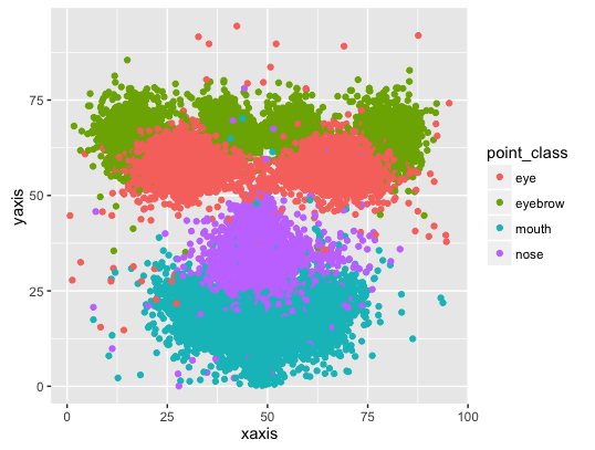
After all the transformations are done, we can concentrate on some simple analysis for the whole image dataset. We can first plot all the key points onto one graph to see the overall distribution of how those key points are located. We can also assign different colors to different key points.
After aggregation, we can see the average key points of all the faces.
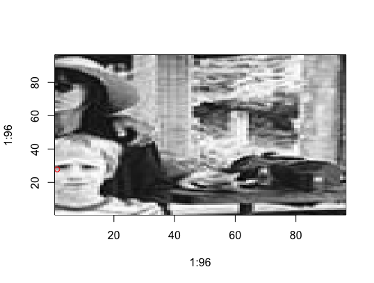
We can see some pictures with extreme points largely deviated from the center.
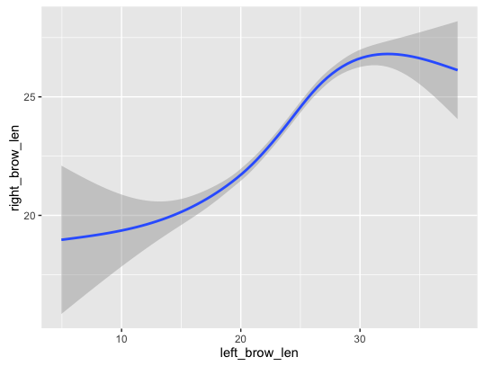
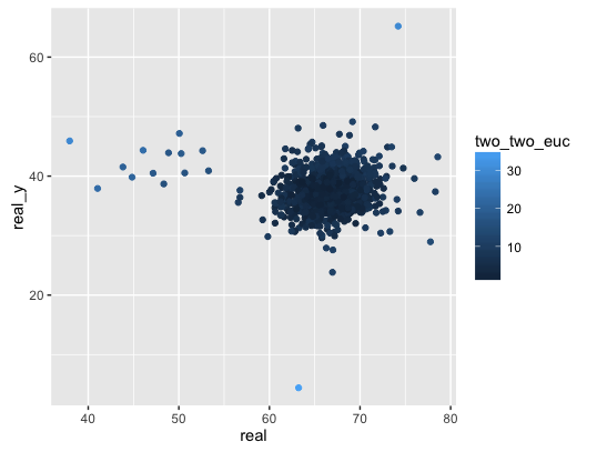
Instead of looking at a single feature, we could analyze the correlation between multiple features. Like Euclidean distance between left eye centers and right eye centers.
Lets make a simple try by assigning all the keypoints of test images the same location, the mean value of all the keypoints in training images. When submitting this online, you will get a very low score 3.96244.
Since the website doesn't give us the answer for the test set, we can build a complete test set by our own through splitting the original training set into two sub sets training and testing. We will split the whole training set through four different ways: 5 equivalent subsets, 10 equivalent subsets, 15 equivalent subsets, 20 equivalent subsets. In each way, one out of the whole subsets would be used as the test set while the others to be the training sets.
Now lets try different splitting methods.
It seems different splitting methods don't influence much on the result. Now let's use a comparatively more complicated method called patching.
Now lets test our models one by one.


