Using Data to Predict Housing Prices in Ames, Iowa
The skills the authors demonstrated here can be learned through taking Data Science with Machine Learning bootcamp with NYC Data Science Academy.
Introduction
Based on data predicting housing prices for consumers and for real estate practitioners can be a useful analysis in many ways. How do you know if you’re getting a “good price” for your house? What aspects of your home most directly correlate with the price? These are the questions we sought to answer, along with finding the relationships between various house features.
We took two different approaches for predicting Sales Price:
- Methodically analyzed each column by data type, checked for correlations and multicollinearity and ran multiple penalized linear regression models.
- Leveraged various tree-based models to pick up on non-linear relationships produced feature importances models performed with high accuracy.
The code can be found here.
Data Description
The dataset comes from a Kaggle competition. It contains 79 features of houses sold in Ames, Iowa between 2006 and 2010, with 1,460 houses in the training set and 1,459 houses in the test set.
The continuous variables mostly describe square footage in different parts of the property along with the age and number of rooms for different categories (bathroom, bedroom, etc).
The ordinal categorical variables describe the quality and condition of the property: the overall, the garage, the basement, and the veneer of the house.
The nominal categorical variables describe things such as materials used, property type, binary features such as whether or not something is “finished” or whether there is central air, and nearby landmarks like parks or railroads.
Exploratory Data Analysis and Feature Selection
We want to avoid the “curse of dimensionality”: when more features are in the data, the data becomes sparser and more spread out among the features, thus making statistically significant conclusions becomes increasingly difficult. Therefore, we need to find a way to choose the variables most important to the sales price and remove or combine any redundant, multicollinear or unimportant features.
Using Data to Analyze Missingness

The above plot shows the missingness of the variables in the dataset. For most features, the missingness is due to the fact that the property did not have that feature. For example, if the house does not have a basement or garage, then all features related to the basement or garage are missing. A small number of features appear to be more randomly missing. The red vertical line at 40% indicates our cutoff used for removing variables with too many missing values. We used this metric to remove the pool quality, miscellaneous feature, alley, fence type, and fireplace quality features.
Using Data to Analyze Imbalanced classes
As shown below, we discovered many of the categorical features were described by only one class within the variable, we ran a script to check for these. If most of the dataset falls in one category, our model may have trouble picking up on the intricacies of the target variable (sales price). If 70% of observations were assigned to the same class of a given feature, then we chose to omit that feature from our analysis.

Using Data to Analyze Skewness

Above are histograms of the target variable: sales price. The sales price is obviously right-skewed (left). To get a more normal distribution, we applied a log transform to the sales price (left). This allows for a better fitting with regression techniques. The following plot shows the skewness of variables in the dataset. Two red vertical lines indicate the skewness of -1 and 1, respectively. We could notice that variables related to porch areas and square footages appear to have high skewness. We later reduce this skewness through some feature engineering techniques. Also, the target variable (sale price) seems to have a problem with a skewness. The above log-transformation on the sale price, nevertheless, can reduce the skewness of sale price greatly.

Using Data to Analyze Correlations and Multicollinearity

Some of the continuous variables and ordinal categorical variables are fairly highly correlated with the sales price. The above heatmap shows these correlations, with darker blue indicating a higher correlation. The sales price is the first row and column in the plot, and one can see that it is most highly correlated with the overall quality of the house, and the ground living area.
These two features are obviously important in determining the sales price. The correlations between the features are also shown: the number of cars the garage can fit and the area of the garage are fairly highly correlated with the sales price with correlations of 0.64 and 0.62 respectively, but they are also very highly correlated with each other with a correlation of 0.88. This makes sense, as a bigger garage should be able to fit more cars. Therefore, one of these variables may be redundant and unnecessary for the data. Similarly, the ground living area is highly correlated to the number of rooms above ground level. In order to remove multicollinear variables, we also ran Lasso and ridge regressions on the data.
After the above analysis, remaining variables are as follows: lot area, house style, overall quality, overall condition, year built, masonry veneer area, exterior quality, heating quality, number of bedrooms above ground, kitchen quality, total rooms above ground, number of fireplaces, garage area, month sold, year sold.
Before moving into feature engineering, we would like to take a look on variables that have high correlation with sale price.

The plot above describes sale price against the ground living area. We notice the strong positive relationship between these two variables. In general, larger living area leads to the higher sale price. Nevertheless, two observations on the lower right corner, which have large living areas but incredibly low sale price, are outliers and we remove them in the later model prediction.

The plot above is the boxplot for each quality level. We could see an obvious increasing trend between overall quality and sale price. On the other hand, there seem to more variations in the sale price for higher quality levels.


Plots above indicate that year and month could make a difference in the sale price. For example, financial crisis was around the year of 2008 and the sale price experienced a minor increase due to the crisis. From the plot of monthly sale price, houses sold in spring tend to have a lower sale price. Because of this difference, we will consider year and month as categorical variables and dummify them before fitting the models.
Feature Engineering and Data Imputation
Aggregated Variables include the following:
“Total area” is the sum of the ground living area and the basement area. The following plot shows that there is a positive relation between sale price and the total square footage ("total area"). As a matter of fact, the correlation between tottal square footage and sale price is close to 0.8, which is higher than any of the individual area-related variabales.

“Total porch area” is the sum of the areas of any porches or decks. As above, the following plot demonstrates the positive relationship between total porch area and the target variable sale price. Though the correlation is around 0.4, which is relatively low. Nevertheless, it is higher than any individual porch area varibles.

“Half baths” and “full baths” were combined from basement half baths/full baths since there was not a difference in correlation with sales price, and these reduce the number of columns. The following plot shows the relationship between the total number of bathrooms (newly-created variable) and the sale price.

Before fitting models, the last step is to impute the remaining variables with missing values. Houses with missing basement features were assumed to not have basements and therefore 0 basement bathrooms and 0 basement area. Similarly, the missing garage areas and masonry veneer areas were imputed as 0. Kitchen quality missing values were imputed as “typical/average”, as that was the median and the mode for that feature.
Models
Using Data to Analyze Elastic Net
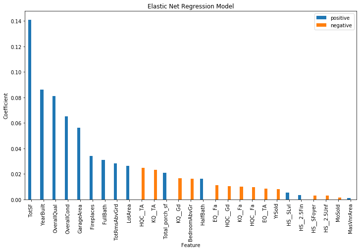
After running a 5-fold cross-validation on the elastic net hyperparameters, we found the best fit to be with a penalization parameter (alpha) of 0.01, and a Lasso/Manhattan ratio of 0.01. The feature coefficients are shown below. While the feature coefficients are not directly interpretable as in an unpenalized regression, the feature coefficients also indicate the importance of each feature in determining the sale price.
The plot shows the magnitude of each coefficient, with the sign given by color. Dummy variables for heating quality, kitchen quality, exterior quality, and house style are given by variables starting with “HQC”,”KQ”, “EQ”, and “HS”, respectively. We can see that the most important features are the total square footage, the year built, the overall quality, the overall condition, and the garage area. This is fairly easy to understand, as a larger house with a large garage that was built recently and is of good quality and condition should cost more.
We used the pace at which the coefficients dropped to zero with an increasing lambda in multiple Lasso regressions to further reduce the number of features. We then ran a grid search on elastic net. This allows us to search for whether to use Ridge penalization or Lasso penalization (rho hyperparameter) and how much of each to add (lamba parameter).
This gave us a training error of 0.1019 and a testing error of 0.1395
Although the testing error is a bit higher than the training error and could point to overfitting, the process we used was very transparent and can be tweaked or changed without losing the entire methodology. We would choose this model to give to a client that doesn’t want a black-box approach.
Using Data to Analyze Tree-Based Models
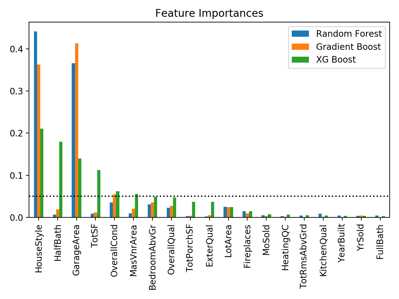
In addition to a regularized multiple linear regression, we also performed a few tree-based models: random forest, gradient boost, and extra-gradient (XG) boost. The feature importances plotted above are for models using the feature selection and engineering described above. The black dotted line marks a feature importance of 0.05.
Both the random forest and gradient-boosted models heavily favor house style and garage area, with random forest only having those two features with importance greater than 0.05, and the gradient-boosted model only also having the overall house condition over 0.05, but just barely. The XG-boosted model shared importance among more variables with 6 variables that have importance greater than 0.05: house style, number of half baths, garage area, total area, overall condition, and masonry veneer area.
For all these models this raises questions: why do the random forest and gradient boosted models prefer house style and garage area over the size of the house, and why does XG boost prefer half baths over full baths? This may be because if two variables have a high correlation or high contingency, tree-based methods may choose either one with little discrimination. House style may be closely related to the size of the house. For example, a 2-story house should be bigger than a 1-story one.
While tree-based models are less interpretable than linear models, they do have one significant advantage: categorical features do not necessarily have to be converted to dummy variables and can just use label encoding. That keeps the dimensionality low and the feature space smaller and therefore easier to fit. Therefore, we added back in most of the variables and reperformed the grid searches.
Below are the feature importances for the 30 features with the highest importance for the XG Boost model. Here, we see that random forest and gradient boost again favor two features, but this time they are different features: lot area and exterior quality. Meanwhile, the most important features for XG boost are overall condition, lot area, overall quality, the fence type, exterior quality, and garage quality.

Conclusions
Below is a table of the training and test (Kaggle) errors for each model. The “v2” indicates fits performed on the dataset with features added back in. Below is a table of the training and test (Kaggle) errors for each model. The “v2” indicates fits performed on the dataset with features added back in. The highest training error also has the highest test error on the random forest model with the more aggressive feature selection.
However, that fit also appears to have the lowest amount of overfitting with a difference in errors of 1.85%, while the rest have at least 3% overfitting. Adding more features lowered the errors in all the tree-based models. The lowest overall training and test errors were the result of using XG boost. This model more equally partitioned the feature importance over the variables, unlike random forest and gradient boost, which probably contributes to its overall better fit.
| Model | MLR | RF | Grad | XG | RF - v2 | Grad -v2 | XG - v2 |
| Training Error | 0.1019 | 0.1253 | 0.1053 | 0.1024 | 0.1145 | 0.0918 | 0.0881 |
| Test Error | 0.1395 | 0.1438 | 0.1353 | 0.1342 | 0.1452 | 0.1340 | 0.1247 |
| Overfitting | 0.0376 | 0.0185 | 0.0300 | 0.0318 | 0.0307 | 0.0422 | 0.0366 |
On the reduced dataset, the multiple linear regression performed similarly to the boosted models. This indicated the overall linearity of the features with the log transform of the sales price. While adding more features created an overall better fit, the main advantage of the linear regression is in its interpretability. It is easy to see how the features relate to sales price. For anyone looking to buy or sell a house, the most important features are overall size, quality, and condition, along with the house style, year built, lot size, and garage size.