Using Data to Predict Iowa Housing Sale Prices
The skills the author demonstrated here can be learned through taking Data Science with Machine Learning bootcamp with NYC Data Science Academy.
Link to the code related to this project: ML_HousingPrices
Data Science Introduction
The goal of this project was to utilize supervised machine learning techniques to best predict housing sale prices in Ames, Iowa. The data set was provided by Kaggle, an online community of data scientists and machine learners, owned by Google LLC.
My team and I worked through the following steps in order to produce a model that ranked in the top 21% of the leaderboard for this Kaggle competition:
- Data exploration and cleaning
- Feature engineering
- Modeling
Data exploration and cleaning
The dataset provided by Kaggle is split between a training and a test set, with each containing 80 categories of housing characteristics data. The training set has 1,460 house sales (rows) of data while the test set contains 1,459 sales.
Missingness Imputation
An initial review of the data showed that there were a large number of missing values across 34 different categories. Below is a graph showing categories that had missing values and the percentage of values missing for each.
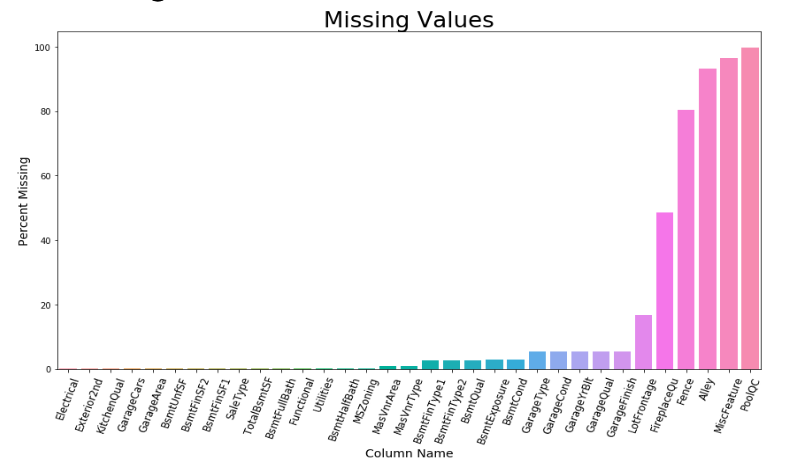
In order to impute missing values, we used a few different methods based on an understanding of the data, the category type and the number of missing values.
The majority of missing values corresponded to the lack of a feature. For example, the missing values in Pool Quality or Alley simply indicated that the house did not have a pool or alley access. As such, we imputed these groups of missing values as "No Feature".
For numerical features with a small percentage of missing values, we imputed using mean or median values, whichever seemed most appropriate. For lot frontage, a numerical column used to account for the linear feet of street connected to the property, there were many missing values. In order to impute these values, we grouped by neighborhood and imputed with the median lot frontage in each respective neighborhood.
We determined that this imputation method would create the most accurate representation of the lot frontage distribution in Ames, Iowa. The only numerical feature not imputed was Garage Year Built, as it had a correlation coefficient of 0.84 with the year the house was built.
Outlier Removal
The final step before working through feature engineering was to check for outliers. Outliers are considered to be values that substantially deviate from the mean and can lead to inaccurate models when used to predict the dependent variable, in this case being the sale price of a home. In the below graphs, you can see five outlier points that clearly do not follow the general trend of the graph.
Houses with an above ground living area greater than 4,700 square feet, lot frontage greater than 300 feet or basement square footage greater than 5,000 square feet were removed from the training dataset, which resulted in the removal of three houses.

Using Data to Analyze Feature Engineering
Correlation Analysis
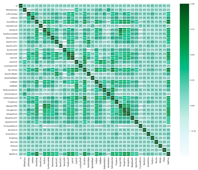
Before creating or editing features, we first wanted to better understand the correlation between variables of the housing data set. The heatmap below illustrates this structure. In this chart, darker colors indicate a larger correlation between two variables while lighter colors show a smaller correlation. The bottom row indicates the correlation between the sale price and the various features included in the dataset. The correlation matrix confirmed our presumption that variables such as overall quality and size were highly correlated with the sale price.
Creating New Variables
One of the most challenging aspects of this project was determining how to handle the large number of dimensions in the dataset. The first task we focused on was creating new variables from the existing ones. The dataset included three different columns which were represented by year: year built, garage year built, and remodeling year. Because the majority of observations had equal values for all three, binary variables were created to capture if there were differences in years.
This would be an indicator that there was renovation done on the home, which could undoubtedly influence the subsequent sale price. Additionally, binary variables were created for houses built before 1960 and after 1980 to determine if houses classified as "old" and "new", respectively, had a significant influence on price. Further modifications of variables are detailed below.

Normalizing Skewed Distributions
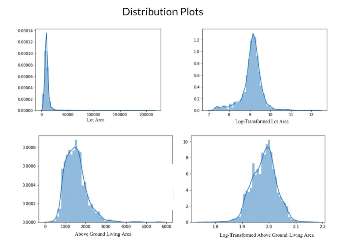
Since normality is an assumption of linear regression modeling, it was necessary to examine the distribution of all variables in the dataset. In order to correct the distribution of variables that were either right or left skewed, we used either a log transformation or a Box-Cox transformation, whichever resulted in a more normal distribution. Below are examples of variables that were normalized, showing the distribution before and after log transformation.
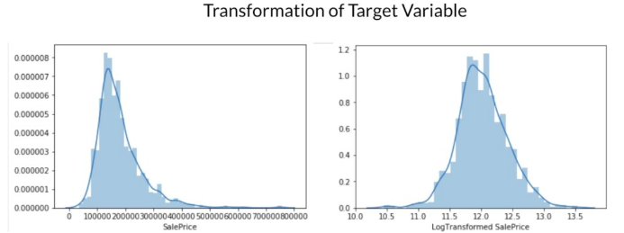
The target variable, Sale Price, was also log-transformed due to its right-skewed distribution.
Using Data to Analyze Model Fitting
Seven different machine learning models were explored in order to produce a model which most optimally predict the target variable, sale price. In order to select optimal parameters for each model, Scikit-Learn's Grid Search CV was used extensively. The three most successful models and our overall results are detailed below.
Ridge Regression
The main parameters to determine in ridge regression cross-validation are the number of folds and alpha. While either 5 or 10 folds are typically the standard, we explored this parameter both visually and numerically to determine which number would be optimal to minimize both variance and error. 10 fold cross-validation was determined to be best in this case.
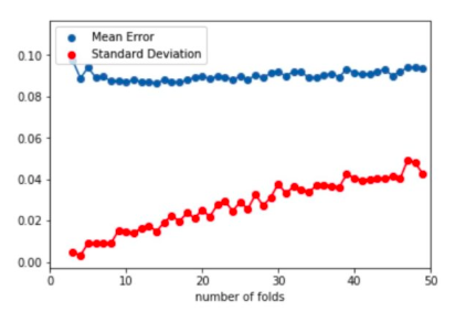
We used an alpha of 10 after running grid searches to determine optimal parameters. This allowed the coefficients to be small enough to avoid over-fitting the training data. As you can see from the below graph, as alpha increases, the coefficients converge (but do not equal) zero.
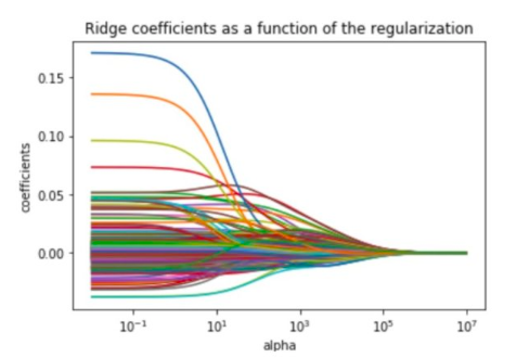
The ridge regression had an R Squared of 0.9418 and a root MSE (Mean Squared Error) of 0.1133, determined by cross-validation and 0.11876, determined by Kaggle.
ElasticNet
The next model evaluated was the ElasticNet algorithm in Scikit-Learn, which is a combination of Ridge and Lasso. The two parameters to tune for this model are alpha and the L1 ratio, which represents the mix between Ridge and Lasso.
The grid search resulted in a value of 0.1 for alpha and .001 for the L1 ratio. As displayed by the graph below, as the L1 ratio is increased, coefficients converge at a higher rate than in the ridge regression, most likely due to the L1 ratio incorporating both the Lasso and Ridge penalty parameters.
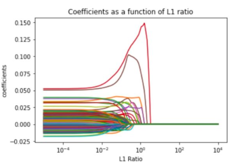
The R Squared value of the ElasticNet was found to be 0.9209, while the cross-validated root MSE was 0.11204 and Kaggle score was .12286.
Using Data to Analyze Support Vector Regression
Lastly, a Support Vector Regression model was built to predict housing sale prices. The three main parameters to tune were gamma, C, and epsilon, which are all related to the level of coefficient penalization. Via the grid search process, we found the optimal gamma to equal 10-6, C to be 1000 and epsilon to be zero. The graph below confirms the grid search's finding of a low value for gamma, and a high value for C in which both result in a low root MSE.

This model produced an RMSE of .11355 in cross-validation testing and .12359 in Kaggle.
Using Data to Analyze Feature Importance: Tree-Based Models
With tree-based models such as Gradient Boosting Regressor and Random Forest, we were able to run feature importance tests to see which variables had the biggest impact on the models. As seen below, Overall Quality, Ground Living Area and Total Basement Sq. Feet were ranked the three most important features for each of these models. While these features were expected to be important because of their high correlation to the sale price, some features we anticipated being important (such as Lot Area) was not deemed as such by the feature importance calculation.

Final Model Comparison
The table below shows the six best models run, include optimal parameters chosen, cross-validation scores, explained variance scores and Kaggle scores. As previously mentioned, the team's ridge model ranked 847 of out 4,086 submissions which placed this study in the top 21% of all submissions!
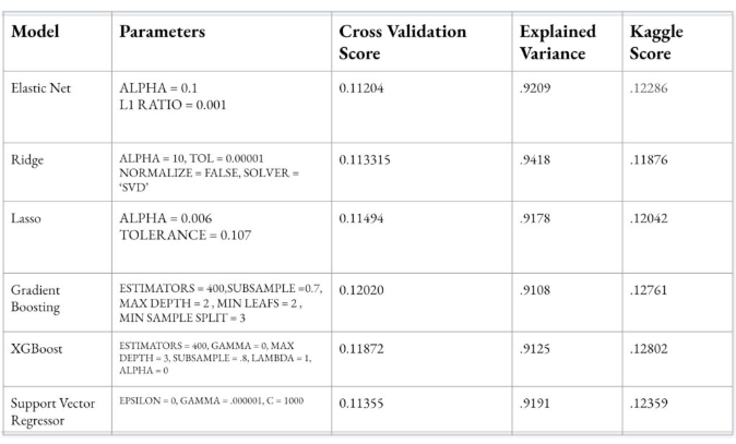
For future work on this project, we plan to experiment further with stacking models, ie combining multiple models to achieve a more optimal result.
Kaggle Competition: Kaggle Link
Please reach out via LinkedIn with any questions or comments. Thanks for reading!

