What Price is Right for That Home? A Machine Learning Approach
Introduction
Housing price is a topic of interest for almost anyone. Being able to accurately predict how much a house can be sold for is of practical importance for homeowners, house hunters and real-estate brokerage firms. With platforms such as Zillow, Redfin, and Compass, the real-estate business has become increasingly more data and technology driven. Domain knowledge from agents are still extremely valuable, yet with the power of rich data and machine learning algorithms, you don’t have to be an expert to accurately predict a house’s selling price.
In this project, we utilized a variety of data analysis and machine learning techniques to predict house prices in Ames, Iowa. The dataset was made available through a Kaggle competition. We finished in the top 15% in terms of prediction accuracy ranking. The modeling shed light on what housing features are important for determining price. Although the high impact factors may differ by market, the machine learning approach is easily transferable. Through this exercise, we also obtained valuable insights into tactical and strategic issues in machine learning projects.
Our prediction efforts followed 4 steps illustrated in Figure 1. This approach was driven by a two-fold purpose: (1) to achieve good prediction performance and (2) to learn ML best practices and techniques. For our team opinion-based subjective feature selection (FS) and feature engineering (FE) turned out to be not beneficial at the beginning stage. We found a more effective approach was to first run models on a “full dataset” with little alterations of existing features except for appropriate imputations and some basic data cleaning. The performance on this dataset then served as a benchmark to improve upon. Feature importance from initial model outputs, together with Exploratory Data Analysis (EDA) and domain knowledge, led to more meaningful FS and FE that improved prediction outcomes.
Note that given additional time one can continue to iterate steps 3 & 4 to improve performance. The entire project was done in python utilizing the sklearn machine learning package, and we used the xgboost python API for xgboost models. Code for this project can be found in my github repository
Step 1: Exploratory analysis and data cleaning
The Kaggle competition provided a training dataset for training ML algorithms and a test set on which submissions are scored. The training dataset contains house characteristics (features) and actual selling price (target) for 1460 houses sold between 2006 and 2010. The test dataset contains records for 1459 houses. The predictions are evaluated by RMSLE between predicted and actual price on the test dataset.
We began with an exploratory analysis to understand each of the variables and potential relationship between variables. EDA was done on the training data, and we made sure to apply consistent data cleaning procedures on the test dataset as well.
We began with an exploratory analysis to understand each of the variables and potential relationship between variables. EDA was done on the training data, and we made sure to apply consistent data cleaning procedures on the test dataset as well.
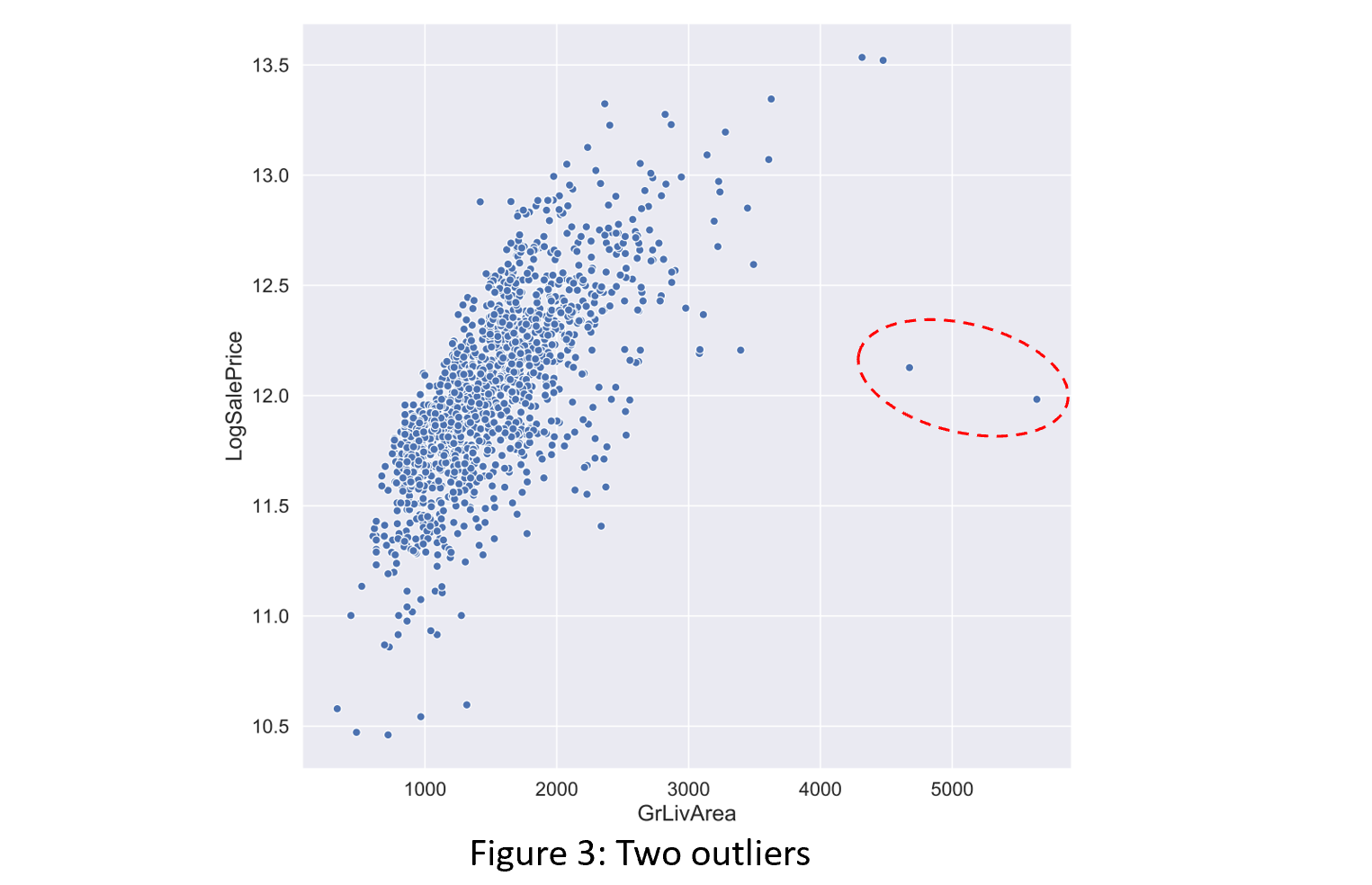
Based on the data author’s suggestion, we removed two obvious outliers shown in the scatterplot below. The actual prices of these two large houses (> 4000 sqft) significantly deviates from the general linear relationship between GrLivArea and price.
Each house has been characterized by 80 features, covering a wide variety of aspects related to the house. Below are a few examples:
- Location & surroundings: neighborhood, distance to highway and railroads
- Size: square footage in basement, above ground, 1st floor, 2nd floor, number of rooms and bathrooms
- Physical condition: material, finish, quality of interior and exterior, year built, year remodeled
- Components, amenities, fixtures: kitchen, garage, central air, fireplaces, porch
- The sale transaction: year sold, whether it was a new construction, type of contract
Some of these features are numeric (e.g. GrLivArea, LotArea, TotalBsmtSF), some are categorical (e.g. Neighborhood, SaleType), and some variables were a type of rating assessment (e.g. OverallQual, GarageQual). We treated most rating-like variables as categorical with the exception of OverallQual. MSSubClass and MoSold appeared as numerical in the data but really should be categorical. We converted them accordingly.
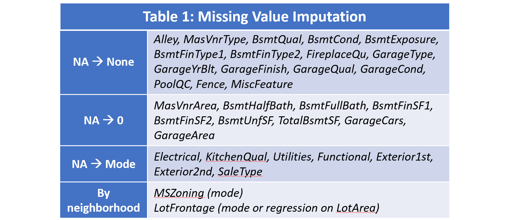
There are a number of features that have missing values in the training and test dataset. Some features have > 90% of missing values (PoolQC, MiscFeature) while others have only a few (MasVnrArea, Electrical). When missing value really means the feature does not exist, we replace NA with “None” (categorical features) and 0 (continuous features). For a few features, we filled missing values with the most common value. We imputed LotFrontage using a hybrid approach. We conjectured that LotFrontage will often have a linear relationship with LotArea, and houses in the same neighborhood may be more congruent in their LotArea and LotFrontage. Hence we ran simple linear regression of LotFrontage on LotArea, by neighborhood. If the fit is good (e.g. R2> 0.5), we use the predicted value, otherwise, we use the median of LotFrontage by neighborhood.
We examined histograms of continuous variables to understand the range of values and shape of distributions. Although many numeric features were highly skewed, we decided to apply boxcox transformation to only a subset where we thought it made sense. Value counts of categorical variables revealed some highly unbalanced variables, providing rationale for eliminating a variable altogether, eliminating certain dummy columns, or combining small categories. We explored such changes in stage 3 of the project (feature selection & feature engineering).
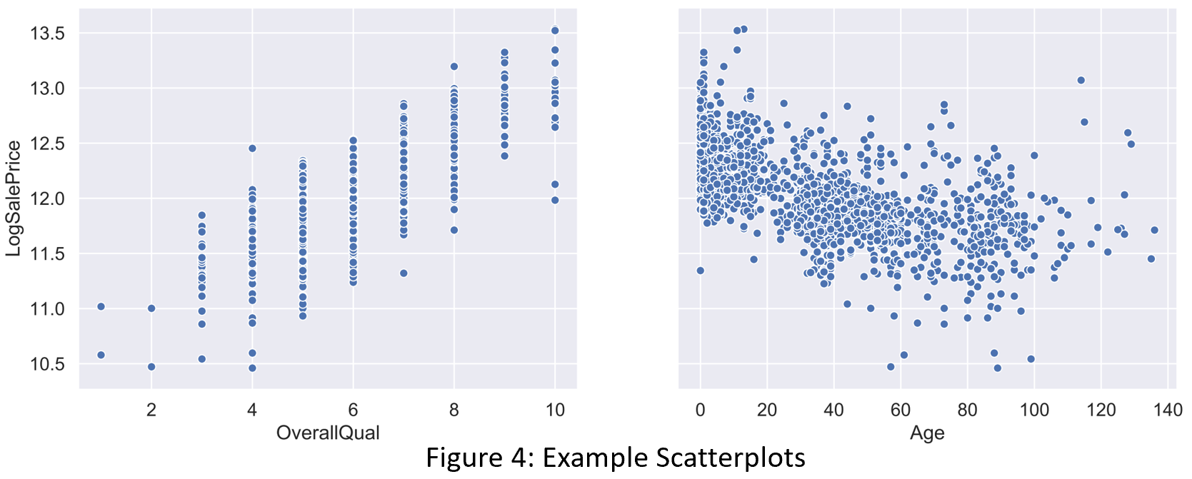
Next we explored pairwise relationships through scatterplots, boxplots and correlation analysis. Shown in the tables above are 19 (out of 38) numerical variables most correlated with price. Size and quality have strong positive correlation with price. In fact, the features circled by dash lines can all be viewed as size indicators. The age of the house, the feature of an enclosed porch, and kitchen above the ground floor negatively correlate with price. Kitchen above the ground could be a proxy for multi-unit dwelling. The scatterplots below verify the approximate linear relationship between OverallQual / Age and price.
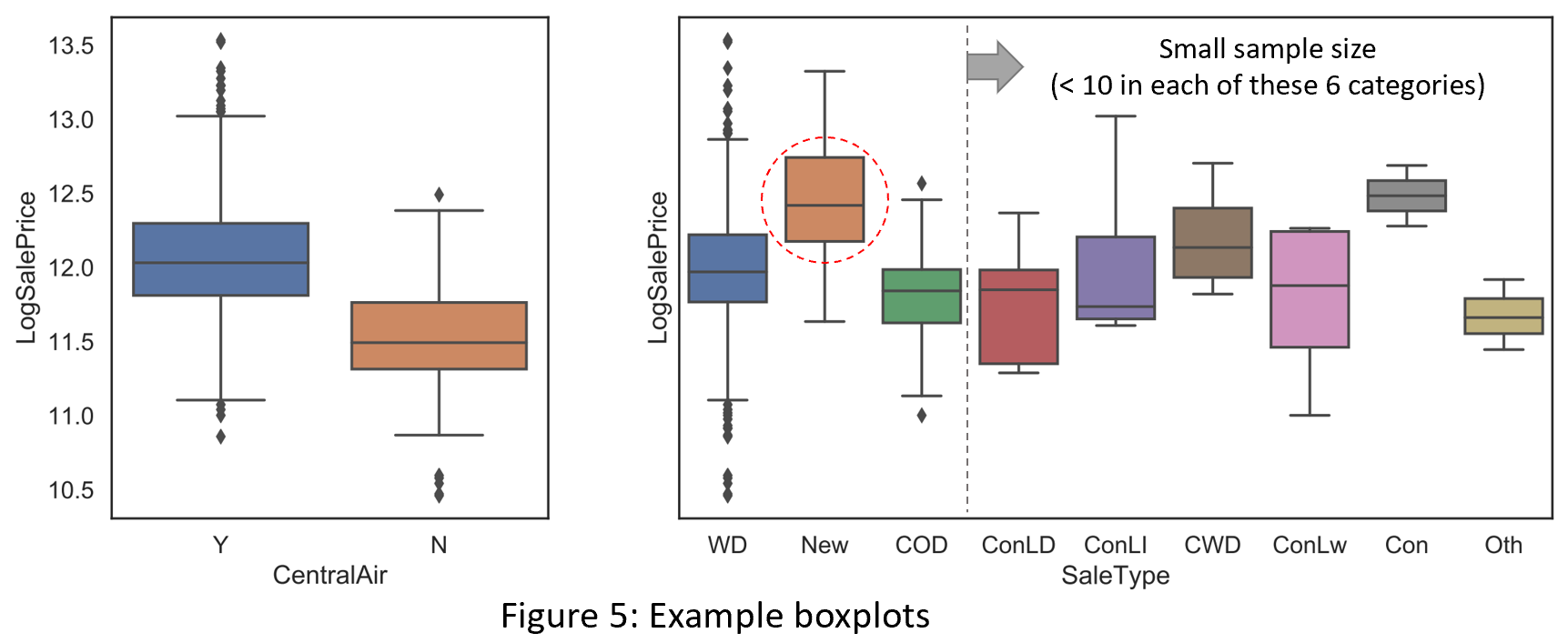
 The relationship between categorical variables and price were visualized using boxplots. Two examples are shown below. The left panel represent a simple case where there is clear separation between the average price grouped by the categories. The right panel is a more nuanced situation. Although there appears to be 9 categories of SaleType, 6 of them have less than 10 observations each. In this case, we can only conclude that houses were sold as new constructions tended to sell at a higher price.
 To investigate further the pair-wise relationship between all the numerical variables, we used a heatmap to visualize Pearson correlation (Figure 6). Indeed, many features are highly correlated, for example: (Age, Re_Age), (BsmtFinSF1, BsmtFullBath), (TotalBsmtSF, 1stFlrSF), (GrLivArea, TotRmsAbvGrd). Similarly, we can visualize the association between categorical variables using a heatmap where the association is measured by Cramer’s V. It’s clear that a lot of redundancy exists among categorical variables as well. For example, the basement features form a cluster with higher pairwise associations, so do the garage features, and exterior features. Neighborhood has significant associations with many features, especially MSZoning.
The overlap between features could present a multicollinearity problem in regression models. This suggests it’s important to use regularization. especially in regression models. At the feature selection stage, it may be beneficial to drop some redundant variables to reduce model variance and obtain more parsimonious models.
Step 2: Model optimization on dataset with full features
Feature encoding and scaling
Using the baseline dataset, we trained 5 sets of models: Lasso, Ridge, ElasticNet, Random Forest, and xgboost. As sklearn models did not handle categorical variables directly, we dummified categorical variables for the 3 regression models and used labelencoder for the two tree-based models. When the cardinality is not high, label encoding is a better approach than dummification for sklearn tree-based models. Dummification tends to make a categorical variable’s importance lower in tree-models, as one variable is split into several.
For the regularized regression models, it’s important to scale the features first. We found that RobustScaler led to better performance than StandardScaler, likely because the former is more robust against outliers.
Model Optimization & Evaluation – Regression models
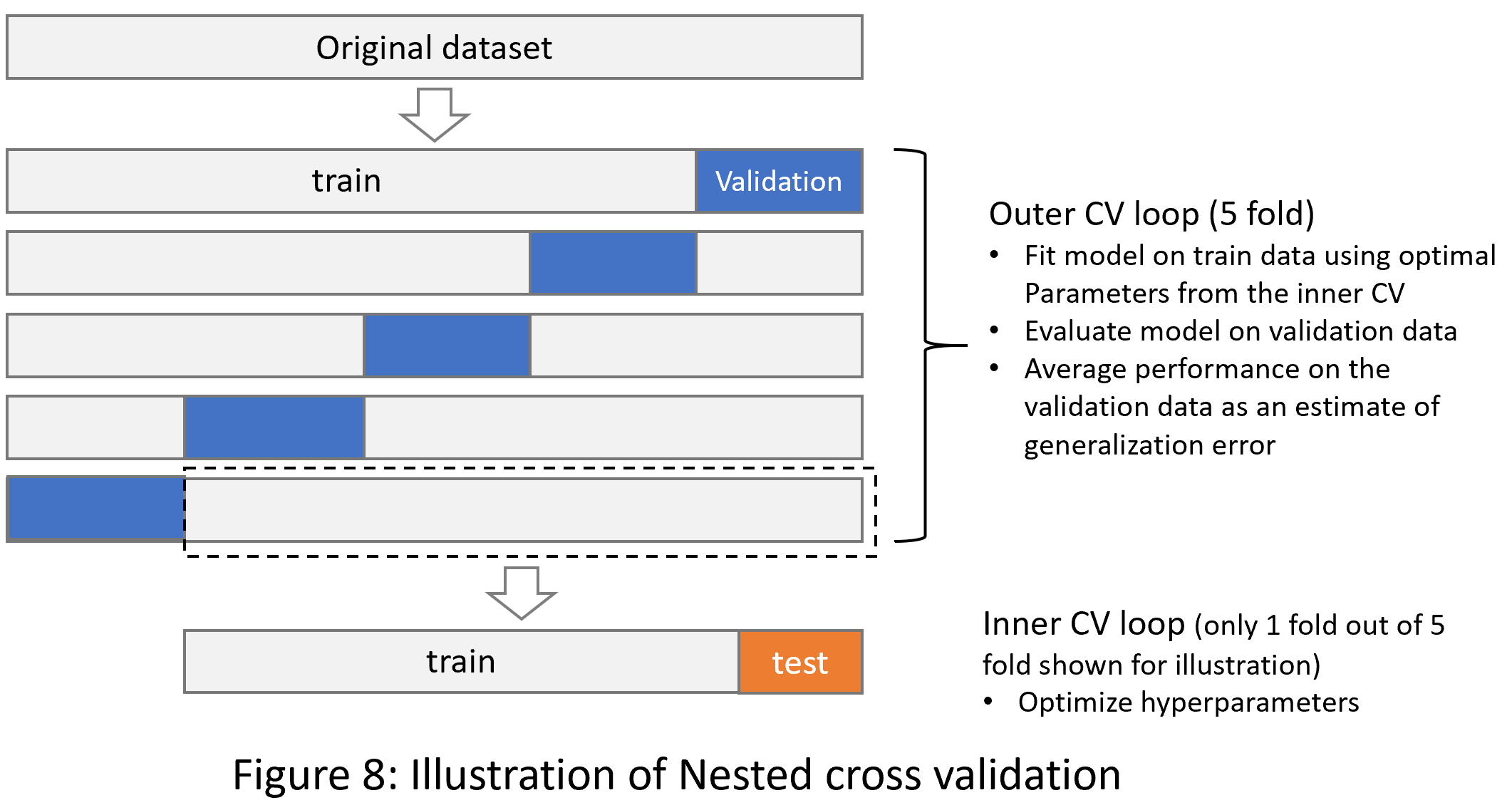
Nested cross-validation (CV) is a recommended best practice for model selection when hyper-parameter tuning is involved. The inner CV loop is used to tune hyperparameters and the validation data in the outer loop provides a gauge for model performance on unseen data.
We used a 5 x 5 nested CV scheme and gridsearch to train and evaluate the 3 regression models. Figure 9 shows the average RMSE on the training and test set from one CV fold on one Lasso model. The optimal regularization strength was between 0.0003 and 0.0007.
 A similar approach was followed to obtain the best ridge and elasticnet models. A summary of model performance on CV and the Kaggle submission are shown in Figure 10. The small gap between all the RMSEs indicate that these models are not overfitting training data and are generalizing well.
Model Optimization & Evaluation – tree-based models
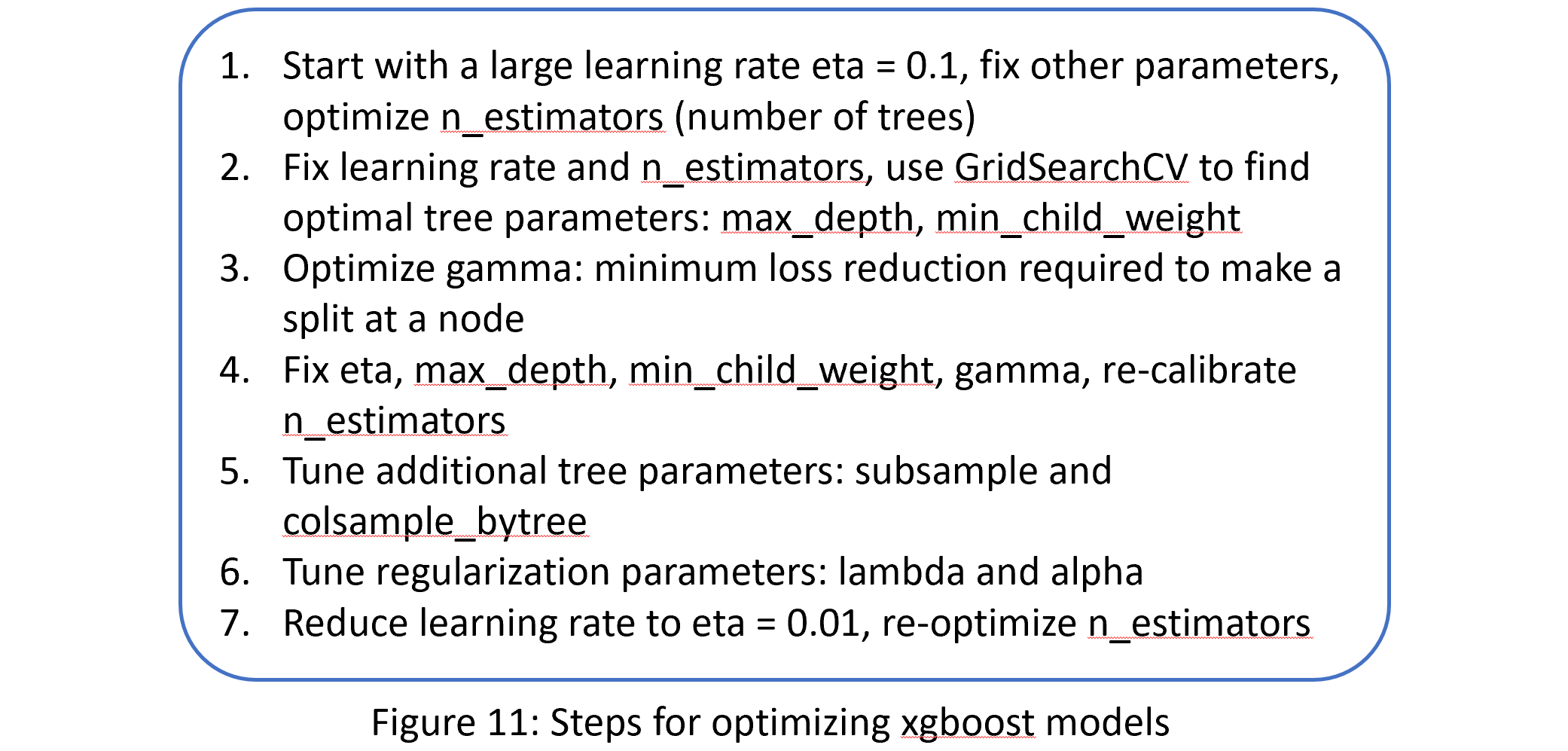
Complex models such as xgboost have a large number of hyperparameters. Tuning those models with GridSearch can be very time consuming. Instead, we followed an approach similar to coordinate descent to optimize xgboost (Figure 11). With the tree-based models, we also simplified by using a non-nested 5-fold CV scheme.
It’s helpful to monitor train/test RMSE as a function of the parameters we are trying to optimize. For example, when optimizing the number of trees in xgboost, we observe the RMSE on training and testing both quickly dropped from 10 to < 0.12 within 100 iterations. However, the gap between the two widens as we increase the number of trees. We allow the increase of n_estimators so long as the RMSE on test set continues to decrease meaningfully.
In Figure 13, the gap between training RMSE vs test or Kaggle submission RMSE shows that overfitting of training data is much more severe on tree-based models than the regression models. Xgboost generalizes better than random forest, given that it uses sequential shallow trees that iteratively fits the residual. Random forest, on the other hand, averages over many larger trees which tend to be correlated with each other. On this dataset, linear regression models capture the relationship between house features and sale price quite well, and performed better (best Kaggle RMSE = 0.11998) than the more advanced models (best Kaggle RMSE = 0.12795).
Feature Importance
Another important aspect of modeling is to understand the feature importance (FI). FI from model output can inform feature selection and help us improve models. In some applications, it’s also crucial to understand the drivers and key factors.
FI can be measured by the regression coefficients in the lasso model. In sklearn tree-based models, FI is typically measured by the total amount of reduction in MSE attributed to splitting on a feature through the model fitting process.
Step 3: Feature selection & engineering
With a model selection process setup, and clear understanding of model performance on a dataset with almost all features retained, we proceeded to experiment with feature selection (FS) and feature engineering (FE).
Our FS and FE efforts were guided by the feature importance from the baseline models and EDA. As lasso performed the best on the baseline data among all models, we focused on engineering features that improves the performance of the lasso model. We made incremental changes to the dataset, and only kept the change if CV performance improved.
We created new features, including recency of remodeling, total square footage, total number of bathrooms, size of good quality finished living space in the basement, total porch and deck square footage, interaction terms between OverallQual, OverallCond with house size, and binary indicators for garage, basement, fireplace, second floor.
We dropped features that showed low importance in models on the baseline dataset, such as Utilities, PoolQC, and MiscVal. We also dropped features that are highly correlated with another feature we kept, and those became redundant after new features were created. Lastly, we dropped dummy variables with extremely low variation across train and test datasets.
We applied two types of feature modifications: (1) box-cox transformations of 5 continuous valued variables to make them more normally distributed, and (2) combined levels of GarageQual that have very few counts and do not have different average sales price when observations were grouped by those levels.
Some of the incremental feature engineering led to improvement of CV scores but not improved Kaggle scores. We kept the changes so long as the Kaggle score did not deteriorate and the change either led to a simpler model or did not increase model complexity in a significant way. The final engineered dataset had 69 features before dummification and 192 features after dummification (vs. 80 and 237 in the baseline full dataset). With the lasso model, we improved our Kaggle score from 0.11998 to 0.11727. This indicates fewer but more meaningful features with less collinearity can lead to better predictions. We can also achieve higher computational efficiency with a smaller dataset.
Step 4: Modeling with engineered dataset
We trained 4 models on the engineered dataset, namely lasso, ridge, random forest and xgboost, following the same approach as we did for the baseline data.
Lasso remains the best model, followed by ridge, and xgboost. Random Forest has the poorest performance. Relative to the baseline dataset, we find the prediction performance improved for all models, as demonstrated by the CV scores and Kaggle scores in table 3. This suggests that all the models benefited from our feature selection and feature engineering, even though we only optimized the features for lasso. Given more time, we can follow the same agile testing approach to optimize features for the tree-based models as well.
From Figure 18, we find many newly created features are among the most important. TotalSF is vital for both models. Age appears to be more important for lasso. The newly created features are more important under the xgboost model than lasso, including two features capturing interaction between size and quality / condition.
Model stacking
Model stacking has been a popular technique kagglers use to achieve winning prediction accuracy. The idea is to create a meta-model based on the predictions from many base learners, each capturing different aspects of the underlying pattern in the data. The simplest model ensembling approach is to take a weighted average of the predictions of base learners in the regression setting or a majority vote in the classification setting. A more sophisticated approach uses predictions from base learners as features to train meta models, with 2 or more layers of stacking (see schematic below). The key to effective model ensembling is to use base models that are not very correlated so that they can complement each other.
We used both a model averaging and a two-layer (base learner + meta model) stacking approach with the 4 optimized base models on the engineered dataset. In the stacking model, we used a multiple linear regression model as the meta-regressor, and the final prediction was also a weighted average of the base predictions. Both simple averaging and model stacking achieved a better Kaggle score than the base learners, improving best RMSE = 0.11664. The improvement over base learners was moderate, likely due to the high correlation between the different base models’ output (0.97 to 0.99).
Future work
Below are some learnings and envisioned improvements we could adopt if we were given more time.
Feature enrichment
The quality of features is central to prediction accuracy in machine learning. ML practitioners have found that cluster membership through an unsupervised ML algorithm such as k-means, when used as an additional feature, can often enhance prediction performance in a supervised ML setting. We could experiment with this technique. Augmenting the Kaggle dataset with additional features such as income, school quality by neighborhood, would likely improve prediction outcome as well.
Hyperparameter optimization
The second improvement would be to use the Bayesian optimization package to tune hyper-parameters. Bayesian optimization iteratively approximates the objective function with a posterior distribution of functions. Bayesian hyperparameter optimization of machine learning models is generally more efficient than grid search or random search. The main benefits are shortened model training time and better prediction performance. It would be interesting to try this approach on the tree-models in this project.
Feature importance (FI)
For tree-based models, we believe permutation-based FI may be more accurate than the native sklearn FI. The permutation approach takes the trained random forest model, shuffles the feature columns one at a time, and compares the out of bag prediction MSE on the shuffled dataset to that on the original dataset. The more important a feature is, the larger increase in MSE we can expect, due to the permutation.
We compared the two FI calculations by running our best random forest model on the training dataset with an artificially added random feature column. Sklearn’s FI ranked this random column #21, while permutation FI ranked it at the very bottom of all features. Fortunately, the top 20 features between the two approaches were generally congruent. We also observed xgboost’s FI ranked the random column in the top 3 to 5 features, which suggests a better approach for calculating FI is necessary.
Categorical variables encoding
We would like to test the tree models in H2O, a Java-based software for data modeling and general computing in a distributed and parallel fashion. Tree-based models in H2O handles categorical variables as is without requiring one-hot shot encoding or labelencoding. This could sometimes lead to better performance than sklearn’s tree models.


