Deciphering the tau tau decay of Higgs Boson
INTRODUCTION
The theoretical discovery and experimental observation of the tau tau decay of Higgs boson is a milestone in particle physics that “contributes to our understanding of the origin of mass of subatomic particles”. Its importance is acknowledged by the Nobel Prize in Physics of 2013.
The Kaggle community also paid huge attention and hosted a data science competition with nearly 1800 teams participating in 2014. The task was to analyze a set of simulated particle collision data containing features characterizing events detected by the Large Hadron Collider at CERN. The objective was to classify events as either a signal indicating the tau tau decay of Higgs boson, or a background noise.
Although this completion was finished almost two years ago, we were still very interested in the Higgs boson Kaggle dataset and wanted to apply our newly obtained machine learning knowledge to analyze it.
EXPLANATORY DATA ANALYSIS AND DATA PREPATATION
Missingness
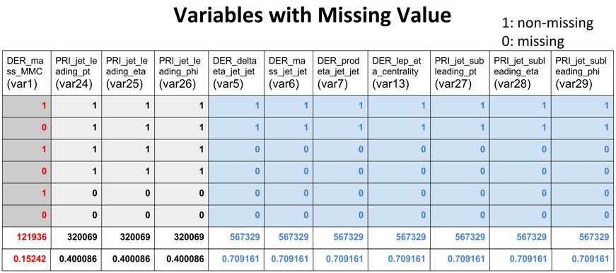
The initial explanatory data analysis helped us identify 11 out of the 30 features have missing values. For convenience, we renamed all the 30 features with serial name from var1 to var30. As shown in the table below, of all the 800,000 observations from the training and test set, there seems to have three systematic types of missingness: 71% have missing values in var5, var6, var7, var13, va27, var28 and var29(Type I); 40% have missing values in var24, var25 and var26(Type II); 15% have missing values in var1(Type III).
Feature Correlation
As shown in the correlation plot below, there are three clusters of correlated variables that are of interest: var4, var10, var12, var20, var22, var24, var27 and var30 seem to correlate with each other; var5, var6, var7 and var13 are correlated; var1, va3 and var8 are correlated.

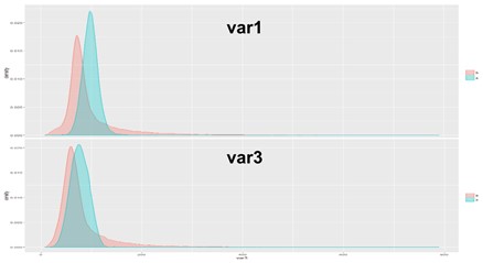
With a further look into the scatterplot with var1 and var3, it seems that there is a strong positive correlation between the two features.

Then we checked the distribution of signal (in cyan) and background (in red) with regard to the two features. It looks like that the two labels have similar distribution regarding the two features.
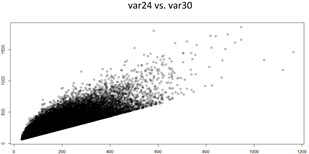
The two graphs below show there are strong positive correlation between var24 and var30, and between var27 and var30, respectively.

Imputation
So why we were interested in analyzing those correlations plots above? It’s because we aimed to utilize those correlation to impute the data. Type III missingness only accounts for var1 and exists in 15% of all observations; Type II missingness shows in 40% of all observations with three features including var24; Type I missingness is available in 70% of all observations and involve 7 features including var27. We would lose much information if we just remove all incomplete features. We used simple linear regression to predict those missing values of the the 11 incomplete features from the 19 complete features such as var3 and var30. Since three of our models were tree based, we were not much afraid of increasing collinearity due to the linear regression imputed features.
Feature Engineering
A combination of those three types of missingness could result in any of the six missing patterns as shown in the table of variables with missing values. If missingness itself is information that could be utilized for predicting the signal, then we should integrate the missingness for modeling. As such we created three dummy variables (0 for missing, 1 for non-missing) to represent the three missing types. Since they are categorical features, their combination could well represent the six missing patterns.
MODELING
Logistic regression:
Since this is a binary classification problem, logistic regression model was first employed due to its efficient computation capability. We built three logistic regression models with different features. The first model uses var1 imputed by a time-consuming Multivariate Imputation by Chained Equations(MICE) method and the 19 complete features. The second model has all the features from the first model and the other ten features which were imputed by linear regression. The third model has all features in the second model and the three additional dummy variables . AIC and BIC were calculated to evaluate the performance of the three models. As the model complexity increases with more features, both AIC and BIC become smaller. It indicates that more features would result in better model performance. The Approximate Median Significance(AMS) score which is used by Kaggle to measure the model accuracy also favors the more complex model with all the 30 features and the 3 dummy variables. In the following modeling, we would use all the 33 features.
| DF | AIC | BIC | AMS | |
| logit.overall.20.variables | 21 | 257665.9 | 257884.9 | 1.95 |
| logit.overall.30.variables | 31 | 249580.0 | 249903.3 | 1.98 |
| logit.overall.33.variables | 34 | 246536.1 | 246890.7 | 1.99 |
Random Forest
Random Forest was an efficient ensembled supervised learning for classification. It operates by constructing many decision trees for training and outputting the class that is the mode of the classification of the the individual trees. It has two important tuning parameters: number of variables randomly sampled at each split(mtry) and number of trees to grow(ntree) to get the best model performance. According to rule of thumbs, square root of the number of variables (5.74)might be likely to be the best parameter of ‘mtry’, so we searched for the best ‘mtry’ around 5.74. We used 5-fold cross validation with different ‘mtry’ values from 1 to 9 and ‘ntree’ values of 100, 500 and 1000.
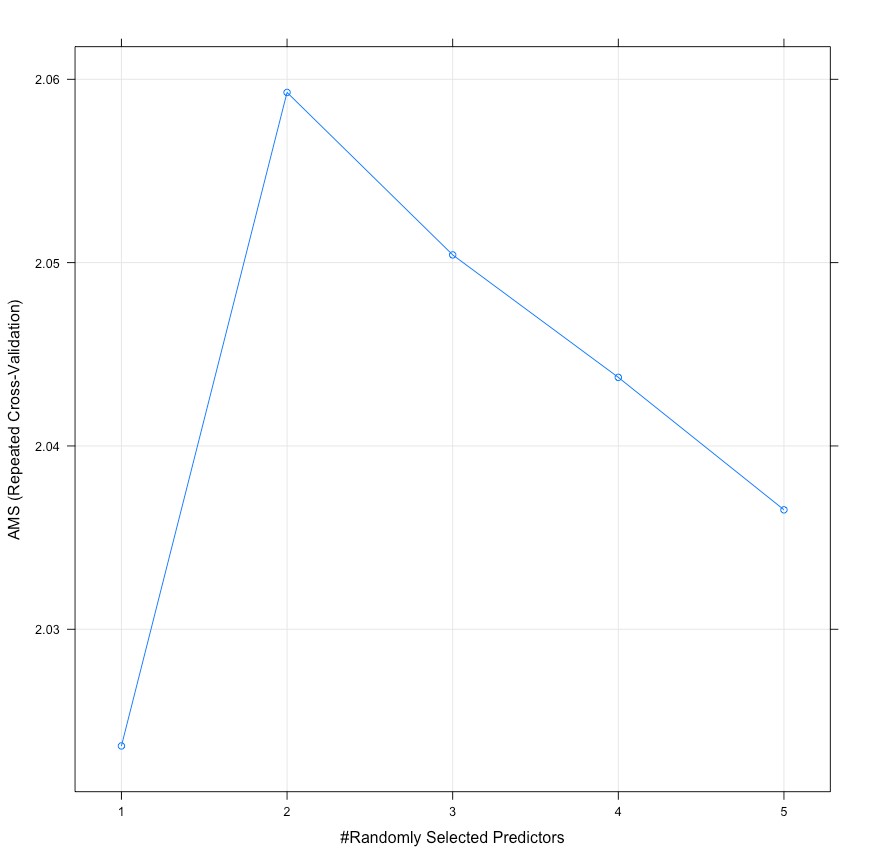

As shown in the graph above, the highest AMS value appears when ‘mtry’ is 2 and ‘ntree’ is 500.
Gradient Boosting Machine
Gradient Boosting Machine(GBM) is another efficient way of tree-based supervised learning for classification problems, which produces a prediction model in the form of an ensemble of weak prediction models. It builds the model in a stage-wise fashion like other boosting methods do and it generalizes them by allowing optimization of an arbitrary differentiable loss function. Instead of building many decision trees (bag of trees) at a time, the boosting procedure generates trees in a sequential manner starting from a shallow tree and then continuously extracting information from the previously grown tree to build a new tree. Since the parameter tuning of gradient boosting is very computationally expensive, we used the default parameter and obtained a AMS score 2.087 in the test set. We used all 33 features as mentioned above, to fit the model.
Here are some parameters worth considering when using GBM:
n.trees: The total number of trees to fit. This is equivalent to the number of iterations and the number of basis functions in the additive expansion.
interaction.depth: The maximum depth of variable interactions. 1 implies an additive model, 2 implies a model with up to 2-way interactions, etc.
shrinkage: A shrinkage parameter applied to each tree in the expansion. Also known as the learning rate or step-size reduction.
n.minobsinnode: minimum number of observations in the trees terminal nodes. Note that this is the actual number of observations not the total weight.
Extreme Gradient Boosting
Extreme Gradient Boosting(XGBoost) is very similar to the regular gradient boosting framework, but it’s more efficient due to the fact that it can perform parallel computation on a single machine, as well as the fact that it uses a greedy algorithm. XGboost supports classification.
Before running XGboost, we must set three types of parameters: general parameters, booster parameters and task parameters. General parameters relates to which booster we are using to do boosting, commonly tree or linear model. Whereas the Booster parameters depend on which booster you have chosen, and lastly the the Learning Task parameters that decides on the learning scenario. In our model we relied on default parameters in the General section of tuning. We focused mainly on tuning our Booster parameters. XGBoost comes with a wide array of different parameters to tune. We focused mainly on tuning those parameters that are generally considered the most important to tune. The 5 parameters we tuned are the following: eta, ntrees, max-depth, scale_pos_weight, and gamma.
Eta : step size shrinkage used in update to prevents overfitting. After each boosting step, we can directly get the weights of new features. and eta actually shrinks the feature weights to make the boosting process more conservative.
Gamma : minimum loss reduction required to make a further partition on a leaf node of the tree. the larger, the more conservative the algorithm will be.
Max Depth : maximum depth of a tree, increase this value will make model more complex / likely to be overfitting.
Scale Positive Weight : Control the balance of positive and negative weights, useful for unbalanced classes. A typical value to consider: sum(negative cases) / sum(positive cases)
We performed a 5-fold cross-validation using the tuning grid.


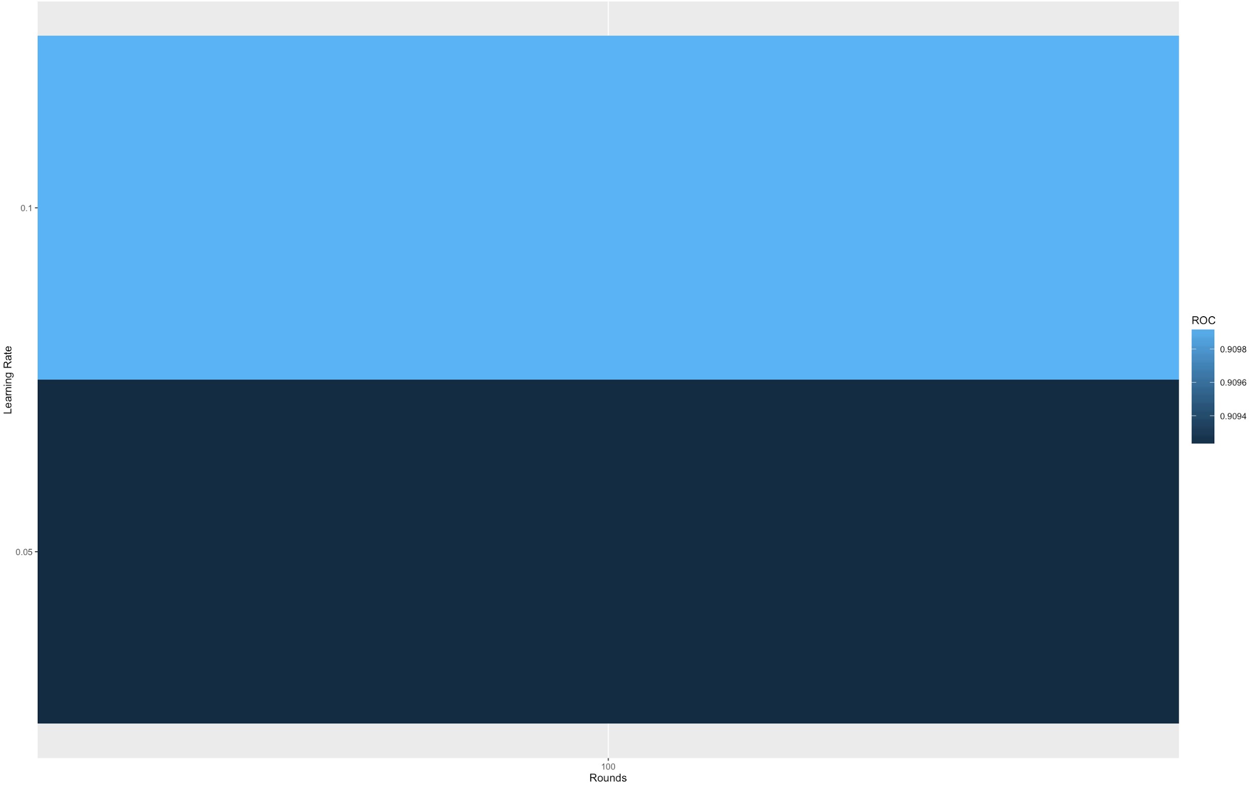
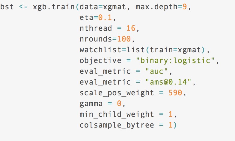
While we did perform cross validation in our analysis, it’s important to note that one of the special feature of xgb.train is the capacity to follow the progress of the learning after each round. Because of the way boosting works, there is a time when having too many rounds lead to an overfitting. You can see this feature as a cousin of cross-validation method. XGBoost allows user to run a cross-validation at each iteration of the boosting process and thus it is easy to get the exact optimum number of boosting iterations in a single run. This is unlike GBM where we have to run a grid-search and only a limited values can be tested.
The XGBoost gave us our best results. We obtained an AMS score of 3.67, and placed 197 on the leaderboard. This was in the top 10% of all submissions.
Feature Importance
Tree-based model would also allow us to draw the feature importance plot based on comparison of information gain of all the features. We drew feature importance plot below and it seems variable var1_d is an important feature which ranks number 7 of all 33 features, indicating the missingness of var1 might be important in predicting the signal.

Ensemble Modeling
Ensemble modeling, combining multiple predictions generated by different algorithms, would normally provide robust predictions as compared to prediction by a single model which only has one individual rule. It’s expected that the diversification and independent nature of each model would improve the predictive accuracy of the ensemble model. From those models discussed above, the XgBoost model seems to perform way better than the other three. When doing ensemble, it’s reasonable to give a better model with more weight. We rank the model by their AMS score on the test set and assign weight 4 to the best model (XgBoost), 3 to the second best( Random Forest), 2 to the third(GBM) and 1 to the fourth(Logistic Model). All the probability predictions on the test set have their rank. The higher the rank is, the higher probability it is signal; the lower the rank is, the higher probability it is background. We could utilize the weighted average to ensemble those four predictive results on the test set and then reorder the averaged result by rank. Based on our best model, the top 14% in rank are predicted to be signal and the rest are background. For the ensemble, we use the same threshold to classify signal and background. The ensemble gives an AMS score of 3.4, which is worse than the XgBoost model which yields 3.6.
Final Results

CONCLUSIONS AND DISCUSSIONS
Conclusion
The Higgs Boson Challenge was a really challenging, yet enjoyable machine learning task. All things considered, we are happy with our best AMS score that gave us a top 10% final ranking. We explored various advanced machine learning methods, including Xgboost, as well as exploring advanced feature extraction methods like PCA.
Limitations
The fact that we only made use of limited computing power definitely held us back. With a lack of proper computing power, we were unable to do extensive parameter tuning — especially when it came to algorithms like neural networks. Another limitations was out lack of domain knowledge required to understand and evaluate the features given. This reduced our ability to select the best pre-processing methods to clean and select data to train the model.
Further Improvements
As mentioned above, we would like to extend our work and incorporate more effective computing power. This will enable us to use neural networks, and stack them with other machine learning algorithm like random forests and boosted trees.


