A.I. Development for Two Sigma Halite II Challenge

Introduction

Halite is an open source artificial intelligence programming challenge, created by Two Sigma, where players build bots using the coding language of their choice to battle on a two-dimensional virtual board. Each game starts off with either two or four players, in which they  compete in a match to either occupy the most planets or destroy the most enemy ships. Each player starts off with the 3 ships and you must dock on planets to gain control and produce more ships.

The purpose of our project was to utilize machine learning techniques to develop a bot which would learn how to play the game. In order to do that, we fed batches of games from the best players into our deep learning models, with the hope that our bot could mimic high-level strategies from the best players’ bots. Below is an example of a 4-player game:

Main Challenges

Our first challenge was to understand the features, outputs, and coding pipeline that was included with the game. These aspects were important for us to build accurate models. Once we understood the framework of the game, we needed to learn how to navigate through python’s tensorflow package and create our deep learning models. Once this was completed, our execution challenges included learning how to deal with the computational complexity of the model and train it in an efficient way. Finally, once the bot was trained, we needed to translate our predictions into game commands and making sure our bot was fast enough in order to avoid it timing out.

Agile Process

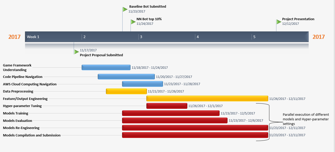
We used an adaptive agile approach that was inspired by Bernard Ong, data scientist and guest speaker for NYC Data Science Academy fall 2017 cohort. The fundamental basis of Agile Process is to maximize the productivity of teams through implementing a divide and conquer strategy in a quick and parallel fashion. By incorporating iterative and parallel tracks, the team can quickly disregard approaches which don’t work and either stick with the current approach or explore other approaches. The idea is to fail fast and move quickly.

What is Agile Process?

The Agile Process is a “standard, industry-wide software development and engineering life cycle, where strategies and solutions evolve through collaboration between self-organizing cross-functional teams”.  Unlike the traditional Agile Process, our modified agile process is designed for machine learning purposes and AI development. Our agile process contains different components but follows a similar parallel architecture to Bernard’s proposed machine learning agile process.

The components for this project included game framework understanding, cloud computing navigation, pipeline navigation and engineering, data preprocessing, feature and prediction engineering,  algorithm selection, hyperparameter tuning, model fitting, model evaluation, model re-engineering, compilation, and submission.

Benefits of Agile Process

In traditional Machine Learning pipeline, each process is executed sequentially; model fitting could only be achieved after feature engineering is decided, and the process of feature engineering could only start after data preprocessing was completed. However, with our agile process approach, we were able to leverage multiple individuals in the team to run data preprocessing, feature/prediction engineering, and model fitting in a staggered parallel fashion. By the end of the first week of our timeline, we submitted our deep fully connected bot which placed us in the top 10%.

Below are some of the approaches that we explored in parallel among the team:

Feature and Prediction Engineering

Feature Engineering was a fundamental component in all of our approaches to improve bot performance in the game. The bot’s performance lies not only in the complexity of the model but what features we feed into the model and what predictions come out of the model. These predictions could then be translated into game commands to the bot. Therefore, we had to constantly update our features and predictions to best suit our approach and improve bot performance.

Some of the features that we engineered to suit our approaches:

Map Engineering and Transformation:

One of the crucial steps before implementing a convolutional neural network is to transform the dimensions of our features into a 3D- array (width * height * num_channels) which then could be fed in batches into the CNN. We came up with 3 different channels: health, ownership, production. The health channel is a 2D map frame array which contains all ships and planet health regardless of ownership. These values are placed in the array corresponding to their respective coordinates in the actual map. Any coordinates which do not contain ships and planets in the map will have a 0 value in the map frame array. Likewise, the ownership channel is a 2D map frame array which has 1, -1, or 0 values. These values correspond to our bot’s territory, enemy’s territory or uncharted territory in the map frame. The production channel follows the same structure as the health channel.

After building the structure of the 2D map frame array, we use min-max normalization to normalize the health and production values to (0, 1) and standardize the size of our map frame arrays. In each game, the size of the map frame changes but maintains the same 3:2 aspect ratio.  By standardizing the size of our input 2D image array into a set dimension (100 x 100),  we can maintain consistency in the output dimension size for each batch of 2D map frame arrays after the convolution and pooling operations in the CNN. We also proposed the idea of mirroring and rotating the input channel frames by 90 degrees to increase the effective data size by 8x.  

K-Means Clustering As Prediction Output:

To make our predictions independent of the game state and applicable to any amount of ships that we have, we utilized the kmeans approach to analyze ship movement. Our idea was to try separate player fleet into up to 10 clusters, so it is easier to analyze and predict the issued commands. After the model is trained it would predict the coordinates of the clusters, and then the ships are distributed to move to those coordinates.

The idea was implemented in our CNN network, but we were not satisfied with its performance and the decision was made to move forward with predicting ships coordinates directly.

Ship Coordinates As Prediction Output:

We also explored the different ways of representing ships positions on the map. The most straightforward way is to use the x and y position provided by the game code, however, this is not a robust solution because the map size is randomized and the prediction will be only relevant for the game with a particular map size.

The better approach is to normalize the map coordinates so that they are ranging from zero to one. Furthermore, we could reshape the map to be the square size, this way we can rotate and mirror it, this way we expand our dataset 8 times.

Another approach is to switch from Cartesian coordinates to polar coordinates. This way, we don’t have to worry about the exact positions of the objects; instead, we can just provide angles and distances between them.

Inputs As Sparse Tensors:

To address the complexity of the network and stay within size requirements and time constraints we decided to transform our input features into sparse tensors and sparse matrices. The reasoning behind it was justified by having large areas of empty space in our map representations. This would also help with data preprocessing times, when we were extracting data from JSONs.

Approach 1: Shallow Fully Connected Neural Network

One of our first approaches was to develop a baseline neural network model and establish a baseline rank for our game bot. We leveraged the template provided by Halite to expedite our approach.The template constructed an architectural code pipeline to develop the game bot as well as provided default features and prediction labels to train the neural network.  Using the template, we built a shallow fully connected neural network on Tensorflow with 2 fully connected layers (12 and 6 neurons in respective layers), 11 default features, 28 prediction outputs, and softmax activation for the output layer. The default features are as follows:

• planet health: integer value depending on planet radius
• available planet docking spots: integer value of docking spots available depending on planet radius
• planet total production: integer value representing total ship production available for the planet
• planet current production: current ship production (positive values for our planet, negative values for enemy)
• planet gravity: total area of influence of the planet

where Ownership (-1,0,1) and ship health (0-255)

• closest distance from planet to friendly ship: integer value
• closest distance from planet to enemy ship: integer value
• planet ownership: 1 for our planets, -1 for enemy planets, 0 for unexplored planets
• planet distance from center of map: int value
• weighted average planet distance to ships:

• planet activity: either 1 or 0 (1 for planets having available docking spots, 0 for none)

The prediction outputs were the allocation distribution of ships to send to each planet on the map (max of 28 planets). The total number of observations is variable depending on the number of games we download and the number of frames in each game. This could be formulated as follows:

Total number of observations = number of games * number of frames* number of planets

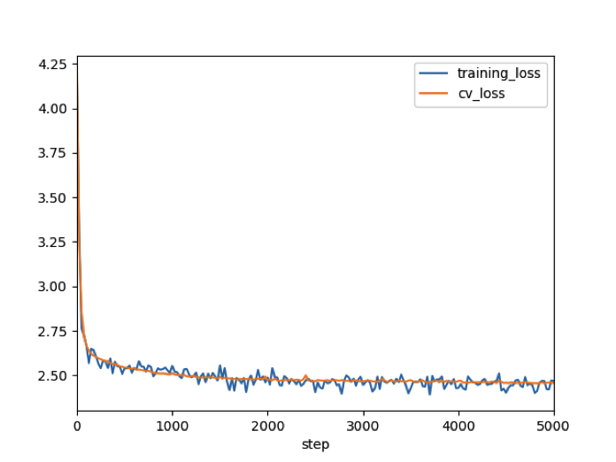
In our case we trained 430 games, a total of 56,014 frames. Thus there were around 1.6 million observations. Above is the cross validation and training loss for our baseline neural network. We defined our loss function to be the cross-entropy loss because of the nature of our prediction outputs as probability distributions. Each step corresponds to a feed-forward and back propagation process and we used 1000 steps to reduce the errors of our weights and biases. Our final cross validation loss was 3.025 and once we compiled the model and submitted the bot, we established a baseline rank of top 70%.

Approach 2: Deep Fully Connected Neural Network

In conjunction to establishing a baseline neural network model, we developed a deep fully connected neural network. The deep fully connected neural network had the same inputs and outputs as our baseline neural network but with different number of layers and neurons per layer. This approach decreased our cross validation loss to ~2.50 and increased our bot rank from top 70% to top 10%.

Hyperparameter Tuning Challenges:

Finding the optimal hyperparameters (number of layers, number of neurons per layer) was a challenge for this approach and subsequent neural network approaches. Machine learning algorithms such as Random Forest and Gradient Boosting can use grid search and bayesian optimization for hyperparameter tuning within a reasonable time. However,  implementing grid search and bayesian optimization for neural networks have significant challenges particularly being time and computationally expensive. These are some challenges for Bayesian Optimization using Gaussian Process with Expected Improvements (GP EL):

• GP EL selects new set of parameters based on the best observation. Neural networks usually involve randomization like weight initialization and dropout during the training process which influences a final score. Running neural network with the same parameters can lead to different scores, meaning that our best score could be due to chance for the specific set of parameters.
• It can be difficult to select right hyperparameters for Gaussian Process because it has lots of different kernel types and even complicated kernels could be constructed using simple kernels as a building block.
• Gaussian Processes are not sparse, i.e., they use the whole features information to perform the prediction. In addition, they lose time and computation efficiency in high dimensional spaces – namely when the number of features exceeds a few dozens.

Because of these drawbacks, we decided to hand tune our hyperparameters (number of layer, number of neurons per layer). We experimented with 5,7,9 layers and 20, 50, 100 neurons per layer and compared cross validation loss for each layer- neuron combination setting for the model. We found that the optimal layer-neuron combination was 7 layers and 50 neurons each layer.

Approach 3: Convolutional Neural Network

A basic model of a CNN, showing the different components involved

There were different design strategies experimented to structure our CNN including network-in-network, skip connections, batch normalization, and very deep networks. Although these methods increased bot performance, the computational cost outweighed their benefits.The most successful architecture proved to be a very simple convolutional network with 2 convolutional layers with leaky relu activations (slope = 0.3), 2 max pooling layers (2x2 and stride of 2) , and 5 dense layers with softmax activation for the output layer. The number of filters per convolutional layer was determined by incrementally increasing it up to a point before timing out became too excessive. At the end of the network,  the default prediction: 28 probabilities of ships to send to planets will be returned.

CNN Performance:

Although the cross validation scores for our CNN model was ~2.3, our CNN bot only ranked in the top 30%. In the early phase of a game, our bot would get stuck in position; going back and forth. We hypothesized that this was due to the lack of early game frame data as well as the nature of our prediction output. In each game turn, our model will predict allocation of ships to send to a planet. These probabilities are turned into game commands which will move the ships in the direction of a certain planet. It happens to be that in early games, there are a lot of different starting combinations that ships can go. With only a few hundred games to train, there is not enough information to capture all the early game ship-planet combination, resulting in abnormal behavior from the bot. Furthermore, if differing game commands are issued in each turn, the bot will exhibit the erratic back and forth behavior.

Future Work:

We had a few things in mind to improve the performance of our model. First, we would eliminate the need for pooling layers in our CNN. Pooling layers help to reduce dimensionality of the array and provides rotational and translation invariance. They are perfect for use in classification situations because they are insensitive to rotations of the image array and the location of objects in the image array. In our case, however, we are not classifying objects in our map frame but we are concerned with the specific location of our individual ships in each turn. Therefore, we do not want to throw away information in that regard. Our prediction outputs would need to be updated as specific coordinates for individual ships to move to instead of allocation of ships to send to each planets. Finally, we plan on rotating and mirroring the image arrays to increase our data size.

Approach 4: Recurrent Neural Network

In traditional neural networks we assume that all inputs and outputs are independent of each other, however, for many tasks this can be a major shortcoming. There are multiple such cases wherein the sequence of information determines the event itself. For these types of cases, we need a network which has access to some prior knowledge about the data to completely understand it. We applied various types of recurrent neural networks as they are especially useful with sequential data because each neuron or unit can use its internal memory to maintain information about the previous input and can handle arbitrary input and output length. In our case, we feed the network a sequence of turns.

Challenges:

One of the early challenges we faced was that the number of frames (turns) varies from game to game. To combat this we used tensorflow’s dynamic unrolling feature, which allowed a dynamic variable in terms of the number of time steps. Internally, it uses a tf.While loop to dynamically construct the graph when it is executed.

The basic RNN design struggles with longer sequences, but a special variant—long short-term memory networks (LSTM) — can work with these. LSTMs don’t have a fundamentally different architecture from RNNs, but they use a different function to compute the hidden state. The memory in LSTMs are called cells and you can think of them as black boxes that take as input the previous state and current input . LSTMs resulted in a slight improvement of score compared to basic RNN network as they were able to include information from the early phase of games. To combat overfitting, we used a common regularization technique, dropout. Additionally, we used multiple combinations of learning rate, training steps, neurons, number of layers, activation functions (relu, tanh, leaky relu).

Gated Recurrent Unit (GRU):

In an LSTM model, there are 3 gates, an input, output and forget gate. This gating mechanism is used to help with longer sequences. Similar to LSTM, GRU models are used to avoid the issue of vanishing gradient. The main difference between the GRU and LSTM model is that GRU only has 2 gates and contains less parameters which make it more efficient and faster for training. Although the performance for the GRU was very similar to the LSTM, this technique allowed us to experiment with different parameters because of its faster speed.

RNN Performance:

The cross validation for our RNN model was ~2.6, ranking in the top 25%. Similar to the CNN bot, the RNN bot struggled during the early phase of the game. We hypothesized that this was due to the lack of early game frames and small sample size (game replays).  However, the bot adjusted in the middle and late stages of the game and on numerous occasions it was able to overcome the poor early game play.

Future Work:

In order to improve the performance of the RNN model, we would like to incorporate a Bidirectional RNN. This model will value past inputs and future inputs in order to predict the current state. We believe that this can help with the early game poor performance.

Blackbox/Tensorboard

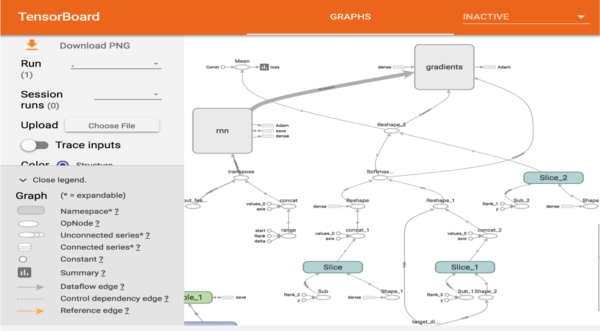
Neural networks are considered to be black boxes: given input, returns output. Internal information about the model, such as the architecture, optimisation procedure, or training data can be hard to visualize and explain to an audience. Tensorflow recently introduced Tensorboard, which makes it easier to understand, debug, and optimize TensorFlow programs. Tensorboard acts like a flashlight on the black box of neural networks by visually breaking down the mechanics under the hood.

We added a lot of details to the TensorBoard so that we can observe while the model trains. Our main intention using TensorBoard was to assist in debugging as well as visualizing the Tensorflow graph to track the various transformations (reshape, transpose etc.). In the future, we plan to use it to plot quantitative metrics and show additional data like images that pass through it such as the input for CNNs. It can also be used to see what the model is learning, especially when the training time increases.

AWS/GPU usage

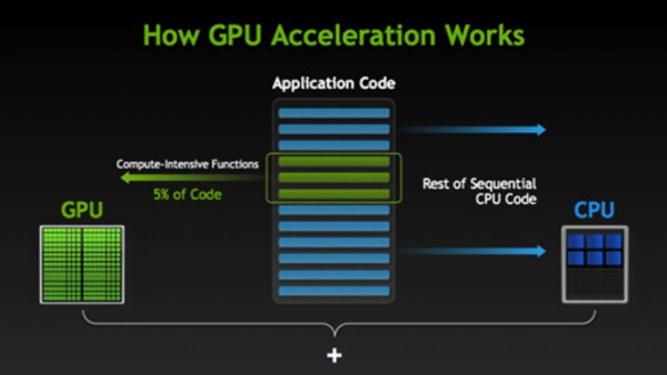
When training a deep learning model, two major operations are performed: feed forward pass and backward propagation. Both of these operations are essentially matrix multiplications of input arrays and weight arrays. While these operations are simple in a mathematical sense, these computations are time expensive when we scale our neural networks (increasing the number of layers and size of our input array). Thus, to compute these expensive matrix operations in a faster manner, we leveraged GPU accelerated computing from Amazon Web Services which offers parallelization of these computations. We were able to connect to the AWS virtual machine and train our deep learning models by launching a spot instance and activating Tensorflow using AWS Deep Learning AMI.

What is GPU accelerated computing?

GPU accelerating computing is the use of graphics processing units (GPU) together with a CPU to accelerate machine learning, deep learning, and engineering applications. They help power and accelerate platforms ranging from artificial intelligence to self-driving cars and drones. GPU-accelerated computing segment computational-intensive portions of the application code to the GPU and the remainder portions of the application code to the CPU. Although GPU cores are slower than CPU cores, they make it up with their large number of cores and faster memory for parallelization of operations. That is why they are suitable for handling expensive computations for deep learning. Meanwhile, CPU by itself is still faster than GPU for sequation code processing.

Atom Teletype/Remote FTP

We were able to maximize efficiency and maintain our agile process through the use of Atom and associated packages, Teletype and Remote FTP. Atom is a free, open source code editor which contain numerous capabilities and packages. One of those packages that we used was Teletype which allows users to share their workspace and collaborate on code in real time. Another package, Remote FTP can edit files directly on a server without having to create a local project. Therefore, we don't have to download the files of the complete project from  AWS virtual machine but simply connect and edit our remote files from Atom. When saving the files, they are automatically updated on the server.

Future Direction

Convolutional Recurrent Neural Networks (CRNN):

One of our future goals is to combine our convolutional neural network with our recurrent neural network. By combining both neural networks, we can take advantage of the feature extraction from CNN and temporal aggregation of features from RNN to generate a more accurate model for our bot.

Reinforcement Learning (Deep-Q Networks):

Our next steps would be to utilize reinforcement learning to create a bot which has direct control over issuing game commands. For this we are planning to use Deep-Q network where we use a combination of reinforcement learning techniques and neural networks to predict expected rewards for each possible action.

Big Data Systems:

To reduce the preprocessing times we could offload the JSON conversion and initial matrix operations needed for feature engineering to big data systems. Distributed computations will help speed up the process and the convenience of PySpark would make it a relatively simple migration.