House Price Prediction with Creative Feature Engineering and Advanced Regression Techniques

Can you imagine that a house can be described with 79 explanatory variables covering (almost) every aspect of a residential home? If that's the situation, then how accurate can the house sale price prediction be, with the state-of-art machine learning technologies? What would be the new challenges arising to advance from the state-of-art to some even further improvement? ... These are some of the exciting questions and opportunities that we have and need to find/give answers to in this project. Specifically, our focus is primarily on

• developing creative and effective feature engineering schemes, and
• exploring and exploiting the potential of advanced regression techniques like random forest (RF), gradient boosting machine (GBM) and model stacking, etc.

Data Set

The project is originated from a house price prediction competition on Kaggle, where the used data set is on the house sale prices of residential houses in Ames, Iowa. For the training set, it gives information of totally 1460 houses, with each house described into 79 variables. There are totally 23 nominal variables, 23 ordinal variables (and thus altogether 46 categorical variables), and 33 numerical variables. The test set contains 1459 house records.

Data Munging

To load such a highly dimensional data set into the work space and prepare it to be ready for analysis is not a trivial task. One particular difficulty we came across is that: many categorical variables just have "NA" as one of their valid levels/values, which really means a certain categorical feature e.g. fireplace, is not available in the house, but have nothing to do with the missingness of data, which is usually what "NA" means in a data set. To handle those false-positive/"faked" NA values properly, we need first import the full data set "as-is" with the default NA finding filter disabled, and then, identify and rename all the false-positive NAs into some name that is not/less misleading, e.g. "None". After that, the true/real NA values are left, for which we can do proper imputations next.

Besides, another complication is that: we need to read from a separate txt file to get information on all the specified data types and categorical levels/values of each of all the variables, and then, can convert each feature variable properly with the corresponding pre-specified data types and categorical levels (whenever applicable).

After that, we checked the missingness of the data set, and conducted proper imputations for the missing values of each corresponding variable, respectively. We followed the recommended right approach of imputing the missing data in training set and test set, completely separately.

Data Analysis

We did thorough data analysis on each of the variable and their respective correlations with the house prices to be predicted. First, the house sale price is log transformed (actually by log(1+x)) to make its distribution better fit with the normal distribution.

For numerical variables, the graph below shows the scatter plots of top 6 numerical features of highest correlation with the house price. We can see that for the first five of them, there are very clear and strong linear relationships.

We also checked the cross-correlations among all the numerical variables. The high correlation coefficients (either ≥ 0.5 or ≤ -0.4) are marked out as follows. This gives us some useful insight to apply PCA (principal component analysis) on those highly correlated pairs/groups of numeric variables, to eliminate multi-colinearity among them, and hopefully may lead to better model prediction performance in the end. This would be one of promising future directions to work on.

For ordinal categorical feature variables, their correlation coefficients with the house price are ordered and shown below. Herein, we can see that some are of very strong correlations with the house sale price, e.g. Overall Quality, Exterior Quality, Basement Quality, etc. while some others may be of very weak/low correlations such as Lot Shape, Fence quality, and Overall Condition, etc. We will show later that for our feature engineering, we picked the top 7 highest correlated ordinal features and converted them into numerical variables and dropped some of the lowest correlated variables, both of which can help improve the model prediction performance.

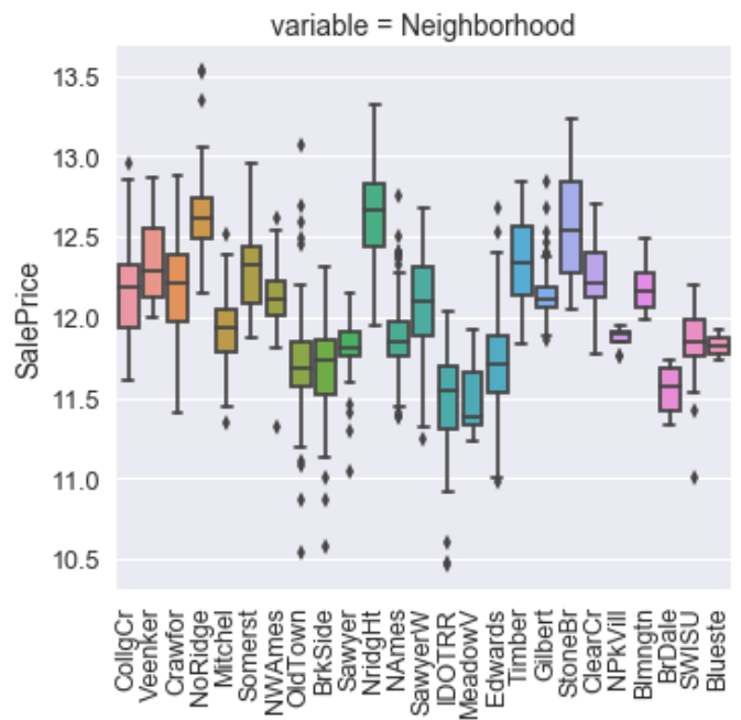
For nominal categorical variables, the box plots below show the house price range variations across different categorical levels/values.  We can see that for the two example categorical variables, i.e. neighborhood and exterior type, house sale prices may vary a lot for different levels/values. This result also implies that these features may have strong impact on the house sale prices.

Feature Engineering

Based on the data analysis results/findings, along with some good intuition or common knowledge on real estates, we conducted our first set of feature engineering steps as follows:

• Identified 7 ordinal variables with very high correlation with house sale price, and converted them into numerical variables.
• Added a "total square-feet" variable as the summation of total basement square-feet, and 1st and 2nd floor square feet.
• Dropped some zero-variance or near-zero-variance categorical variables (i.e. almost all of the same categorical value/level).
• Handled time related variables properly, e.g. garage year built, year built, year sold, month sold, to better fit for regression.

The major ideas/logic behind them are:

• Reduce the number of categorical variables whenever possible/appropriate, as each categorical variable will have to be converted into multiple dummy variables for regular multiple linear regression model (a.k.a. ordinary least square (OLS) model) and regularized linear regression models, e.g. Ridge, Lasso, and ElasticNet, which would greatly increase the total number of variables and become very inefficient on prediction.
• Add new promising feature variables based on domain knowledge.
• Remove trivial variables of very low prediction value.
• Adjust variables properly as needed to make sure their values or types are well fit for the purpose of regression, i.e. help to accurately predicting the value of the target variable.

To seek more feature engineering possibilities, one effective approach we found and used is to conduct feature importance analysis and feature selection with the help of the Caret package in R, and applied the result for feature selection in our actual modeling process with Sklearn in Python.

Specifically, we first ran RF model fit on the training data in R, and collected feature importance info of all the variables. Then, using the recursive feature elimination (RFE) function from Caret, we sorted all the feature variables from the most to least important, and conducted backward selection of features via dropping 5 variables at a time, and compare their cross-validation (CV) prediction performance. As such, we can find the optimal feature set that gives the lowest RMSE (root mean squared error) prediction error. The result figure is shown below, which shows the dropping of 10 least important variables will give the best RMSE performance.

As another alternative approach, we then inserted two new noise variables into the feature set, i.e. one standard N(0,1) Gaussian distributed noise variable, and one standard [0,1] uniform distributed noise variable, and ran RF to check the feature importance again. The intention herein is to see how the importance of all the actual feature variables looks like compared to the importance level of the two noise variables as good importance indicators/markers, such that variables of importance level below those of the noise variables, will be considered good/promising candidates of un-important features to be removed.

In practice, we found that the insertion of two differently distributed noise variables as mentioned above is quite helpful/important in that: with different RF model tuning parameters, e.g. the number of randomly selected feature variables at each step of tree split (denoted as "mtry" in Caret), the actual ranking of the two and their relative positions to each other may be changed quite dynamically. E.g. for one mtry value, Gaussian noise variable importance level may be much higher than the uniform noise variable, which is actually of the least importance level among all, and thus on the very bottom,  but for another mtry value, the uniform noise variable may be instead of higher importance level than that of the Gaussian noise variable, and both are away from the bottom level. Therefore, we found that using two differently distributed noise variables serves well as a robust approach to pick out un-important feature variables. In this way, we identified another set of 9 variables in addition to the 10 selected variables from backward feature selection earlier.

These two sets of variables become our candidate sets of dropping variables to test in the next model tuning and selection process. Note that for non-parametric decision tree based models like RF and GBM, it is not necessary to convert categorical variables into binary dummy variables. Especially, for Caret in R, with the total number of levels of a categorical variable less than a limit (i.e. 53), the RF model can just directly take those categorical variables as inputs for the regression, while for Sklearn in Python, we still need to use LabelEncoding to randomly map categorical levels into numerical values to convert one categorical variable into one numerical variable with multiple values. However, both will definitely yield better modeling performance than the dummy variable conversion.

Unfortunately, we didn't realized this point in the very beginning, and training different models with different set of feature variables adds extra implementation work, which we cannot make it in the limited time frame of the project. So, in our model tuning and selection process, we still convert all the remaining categorical variables into dummy variables as inputs, which inevitably increases the total number of variables from 79 to 218. We mark down this direction as one of the future works for further improvement in the end.

Model Tuning, Selection, and Stacking

We used 80% to 20% split of the original training set for the actual local training set and test set, respectively. For linear models, we tried and tested with the regular OLS model, and the regularized linear models of Ridge, Lasso, and ElasticNet. For non-linear models, we tried RF and GBM. For model tuning, Sklearn's grid search with CV function is used to find the optimal hyper-parameter values. Moreover, for the tuning of GBM model which involves a lot more number of hyper-parameters than the other used models, instead of purely relying on exhaustive grid search without any human supervention/interaction, we found and followed a reasonable approach efficiently combining grid search with proper hand tuning.

For single model selection, we found that the best performed single model is ElasticNet, whose best tuned hyper-parameters are alpha= 0.1833, l1_ratio=0.015, meaning more toward l2 norm of Ridge. Result shows that it only uses 32% of the total feature variables.

For model stacking, we used the typical averaged model stacking paradigm from Kaggle, and finally tested and chose to stack the best tuned ElasticNet, RF and GBM models altogether. Although the prediction accuracy of the stacked model is a little lower than the best single ElasticNet model on the local test data set, when actually uploaded to Kaggle for a much larger test set (1459 rows) testing, the final Kaggle score of stacked model is better than that of the single best tuned model of either ElasticNet or GBM. Therefore, in our experiment, the stacked model performs the best.

We tested the feature selection idea of dropping the two candidate sets of selected low importance variables, one at a time. Result shows that such dropping always improves the prediction accuracy for all the linear models of OLS, Ridge, Lasso, and ElasticNet. For GBM, the performance degrades a little, but after re-tuning the hyper-parameters, its performance also becomes a little improved than before. Except for RF, even after model re-tuning, the performance is still a little worse than that before the feature dropping. In spite of that, as we tested, the overall stacked model performance is also always improved by the selected feature dropping. Therefore, this result confirms the effectiveness of our feature selection approach.

The final achieved model performance of all the tested models for the local test set are listed as follows.

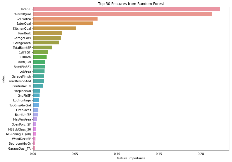
Result of top 30 important features collected from best tuned GBM and RF models is shown as follows. Due to their different learning behavior, the resultant feature importance results are also different. While GBM's feature importance is more evenly distributed among different features, in contrast, RF's feature importance is more concentrated on a fewer number of highly important features.

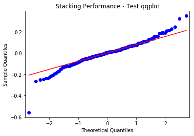
Finally, some graphs on the final stacked model performance on the local test set are shown as follows. We can see that the model performs reasonably well without much serious violation issues on constant variance, normality, and independent error, etc. Note that starting and ending portion of the qqplot are not so well fit for the normal distribution. We think that this is more or less due to our having not carefully checking and removing some of the outliers from the data. This is also marked down as a work for future improvement.

Conclusions and Future Directions

This project is really a great learning experience, which lets us going thorough the whole entire process of building a machine learning model to solve a practical regression problem in real world, starting from the very beginning of data analysis, cleaning, preparation, etc. till the model stacking, evaluation,  and delivery in the very end. We touched upon, thought over, and finally either solved or gained useful knowledge/understandings of many sorts of major or minor practical issues, which is really a very rewarding process overall. In the end, we all agreed and realized that: feature engineering is more often than not one of the most critical part or differentiator on the final model performance.

Due to limited time, we realized but have no time to try many of the interesting/promising directions/ideas, which are summarized as follows for a good reference in the future.

• Try other advance models: XGBoost, SVR, etc. and tune with Bayes Optimizer
• No need to convert categorical variables to dummy variables for tree-based models (H2O RF, etc.)
• Try using different feature selection for different models: i.e. only dropping features for linear models, but not for tree-based non-linear models
• Try more preprocessing choices as BoxCox transformation, PCA, etc. For PCA, we may use the cross-correlation result among all the numerical variables, as shown earlier, to find highly correlated groups of variables, and only PCA on them and see.
• Outlier check and removal
• Clustering analysis to generate new useful categorical features
• Feature selection: try other advanced algorithms e.g. Genetic algorithm, and simulated annealing, from R Caret package.

(All the code, data, and presentation, etc. can be found on GitHub.)