Kaggle Competition: Allstate Claims Severity
1.Introduction
Allstate Corporation is one of the largest insurance companies in the United State. The main products that Allstate offers are car insurance, recreational vehicles insurance, home, property, condo, renters insurance, and so on. In order to provide better claims service for Allstate’s customers, the company is developing automated methods to predict claims serverity. Allstate launched this challenge on Kaggle, and invited all the Kagglers to tackle down this task with their technical skills and creativity.
The goal of this challenge is to build a model that can help Allstate to predict the server of the claims accuratly. At the same time, to provide the important factors that have strong impact on the severity. With these information, Allstate can proposed or adjust more suitable insurance packages for their customers.
On top of this, as a team, we wanted to implant the data manipulating, features engineering, and the machine learning skills that we have learn to perform a strategic process, and established a model that has strong capability to achieve the best prediction possible.
2.Workflow
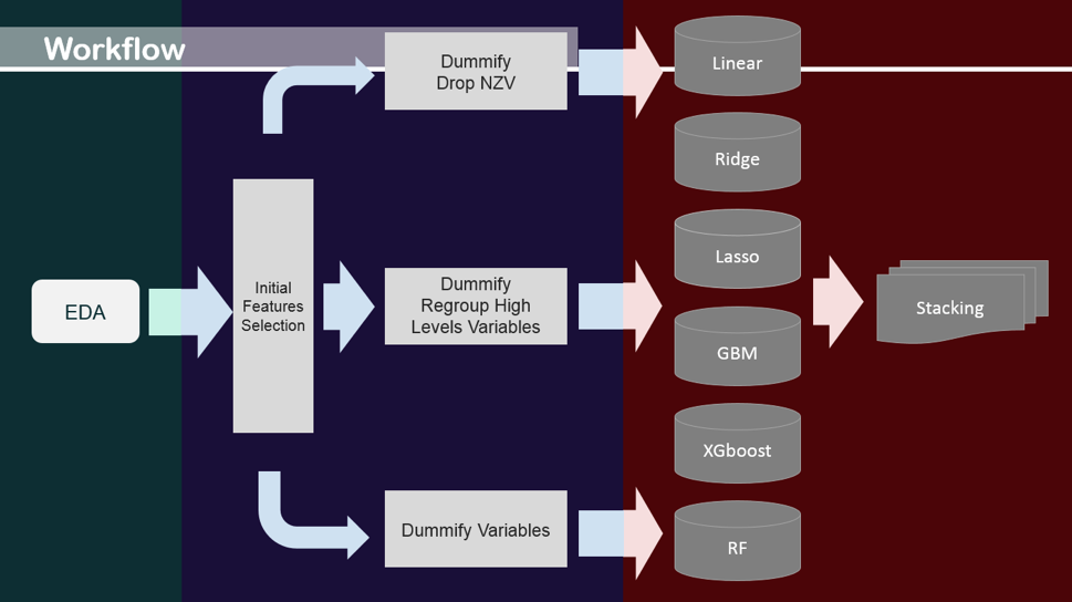
In order to tackle down this challenge within two weeks as a team, we were following the pipline showing above from the begining. The workflow is dividing into three main parts:
1) Exploratory Data Analysis (EDA): Due to all the features are annonymous, EDA became a very important stage for us to understand more insights of the data. This stage is also crucial for the next stage - Feature Engineering
2) Feature Engineering: Feature Engineering is the stage that allow data scientists to exert their creativity. It is also the stage that can help to differenciate the models from others. For the initial features selections, we decide to use unsupervised learning methods, PCA and K-means to see is there any possibility to reduce dimensions and cluster the features. After the first attampt, we also used three different encodi09ng methods:
- Dummify the categorical variables and keep all of them
- Dummify the categorical variables and drop the variables that have near zero variance
- Dummify the categorical variables and releveled the variables that have high numbers of levels.
- Model implementing: the third stage is implementing single models and fine-turning them. From there, we have selected the best performing models to do model stacking.
3) The models we have used are:
- Multiple Linear Regression
- Ridge Regression
- Lasso Regression
- Random Forest
- Gradient Boosting Model
- XGBoosting
3.EDA
The complete training data set contain observations, 130 continuous and categorical input variables, and 1 continuous output variables with no missing value. The density plot of loss below provide the information about the distribution of the output variables. It indicates that the observation is skewed to the right. To prevent high leverage from the outliers, we did a shifting and log transformation on ‘loss’, so it can be more normal distributed without changing the order. Second density plot is the result after traformating the output variable.
From the numeric graphic analysis, it inicates that the data set has 116 categorical variables and 14 continuous variables for the input features. For the categorical variables, the lowest number of levels of variables is 2 levels, and the highest number of levels that appears in the variables is 326 levels. With such high number of levels in the variables, this is the part will be focused on during the feature engineering. After further investigation, another import information about the categorical variables is that some variables containing levels only in the test set, but not in the training set. The chart below lists out the unique levels for the categorical variables that have this behavior.
For the continuous inputs, the correlaiton plot provides the insight among the variables. The plot indicates that there are some strong relationship between some variables. This is important information for building model later on.
4.Initial Feature Selection (PCA, K-means)

In order to explore the potential dimension reduction, the unsupervised machine learning methods PCA and K-means were applied to the training set. Based on the resurlts of the scree plots from PCA and K-means, the dimensions are not able to have a siginificant reduced. For PCA, with about 48 princial components, around 88% variance is explained, under 95%. For K-Means, even with 20 clusters, the within-cluster variance is still very large. As the result, we have to move forward with other feature engineering methods to improve the accuracy, and reduce the computation expenses at the same time.
5.Feature Engineering
In this project, we did three different types of feature engineering. The findings form EDA showed that there are more than 100 categorial variables in this dataset. Most of them have two levels, which is fine for modling. However, a few of them have many different levels; some of them have levels greater than 100. So, we did a dummy transformation first. We broke categorical variables with many levels into several dummy variables. It means that for a categorical variable, when one of its levels have one observation, it becomes a dummy variable having (n-1) zeroes. Hence, after the first step, there were many dummny variables which were near zero variance (NZV) predictiors. We could keep all of them or drop the features which had NZV. , we used both of them to build models, however, the results were not good.
On one hand, removing data should be avoided, if possible. We were not sure if the NZV predictors wrere non-informative. Those NZV features could in fact turn out to be very inofrmation. However, keeping all of features took us long time than expected to build models, and it might result in overfitting as well.
On the other hand, we used the function nearZeroVar from the Caret package to remove NZV predictor. By default, a predictor is classified as NZV if the percentage of unique values in the samples is less than 5%. The advantage was that this method saved us a lot of time to build models, however, the drawback was that it increased the error and resulted in losing some potentially important information.
In order to balance between time consumption and error reducing, this project regroups those categorical variables over 15 levels, to keep as much information as possible. After regrouping, this project dummifies the new categorical variables with the rest for the third round machine learning. The good thing in this way is that useful information is kept. However, there are multiple ways to group variables.
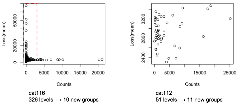
Let’s first explain the reason why 15 levels here is a good cutting point. When using near zero variance to drop features, for categorical variables, it removes those levels with less than 5 percent of observations. For such a large dataset, 5% means around 9500 observations. Even if a level having 9000 observations, which must have some useful information, will be removed from the dataset. For variables like cat116, which has 326 levels, only 3 levels are kept after near zero variance feature engineering. Even in an ideal case, only 19 out of 326 levels can be used for the further machine learning, which is certainly not desirable. Meanwhile, this ‘ideal’ situation also tells the fact that 20 is not a good cutting point. To be more conservative, this project determines to regroup categorical variables over 15 levels. In other words, keep over 5 percent of observations in each level.

Here are two graphs. Each graph represents one categorical variable. Each point here is one level. The x-axis is counts. That is how many observations in each level. The y-axis is mean of the loss for each level. An interesting finding is that, in most cases, the scatterplot is like two straight lines, one vertical, one horizontal, like in the left graph. The right graph, Cat112, is an exception.
However, the ways to regroup are using the same idea: first, keep the original levels having over 5% of observations, and then split them based on the average loss and counts, regroup them into high loss, low count group, low loss low count group, low loss low count group, and so on and so forth.
By doing feature engineering in this way, it also manually builds a connection between loss and those categorical variables. The next step is the third round of machine learning.
6.Models:
6.1 Linear Regression
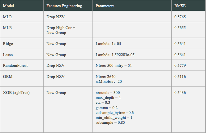
The first individual supervised model we tried was Multiple Linear Regression. We mainly used this model to check would there be any difference between different feature engineering methods. The Linear model had been tried on 3 encoding methods. The first encoding method did not go through due to high number of variables has 0 variance. After dropping the variables has near zero variance, the model gave the RMSE around 0.57659.
On top of using the third encoding method, which was to relevel the categorical variables that had high number of levels, we also droped the highly correlated continuous variables to test. The model returned the RMSE around 0.56557 this time, which indicated that the third encoding method performs better on the linear model.
6.2 Ridge & Lasso Regression

Based on three types of feature engineering, the new group gives the best results. In ridge regression, the best lambda is 1e-05, and the RMSE is 0.56414. In lasso regression, the best lambda is 1.592283e-05, and the RMSE is 0.56415.
6.3 RandomForest
For the random forest model, we used the data set from second encoding method, which is drop the variables have near zero variance. The default setting was used for the initial fit, which is 500 trees, and 51 mtry. However, the model took two days to finish the training without cross validation. Due to high computational expenses, we choose to move forward to other individual models.
6.4 GBM


Three Gradient Boosting model were trained:
- the variables with less than 5% variance were removed
- all the variables were ustilized for the model
- reduce the levels of category variables
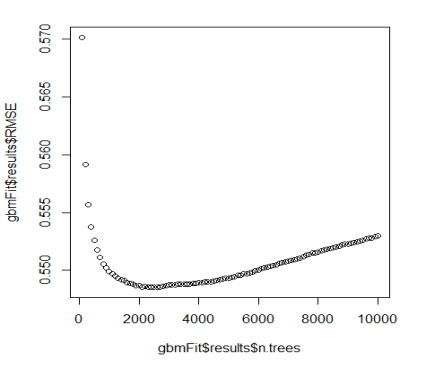
Four parameter were cross validated based on the subtest data, such as ntree (number of trees), shrinkage factor, depth of trees and number of the minmun obersevation in the nodes(figure 3&4),From the models with the best parameter, the model 2 show the best accuracy (RMSE 0.51)but expensive computation(3 days), the model1 lower accuracy(0.54) but efficient(1.5 days),and the model3 sufficiently appoach the balance of the accuracy(0.53)and the computation(2days).
6.5 XGBoost


We also tried XGBoost from Caret package to build models. Similarly, the new group shows the best results. Compared with running XGBoost package directly, the XGBoost from Caret already reduces the total number of parameters people can tune to seven. After trying different combinations of parameters, we found that there were two of them really affected the model, which were nrounds and max_depth. The rest were less relevant. The left graph above shows the result of the cross validation which gave us the best model, the corresponding smallest RMSE is 0.5436. Meanwhile, the most important feaure is cat80D (see also right graph above), also similar with the results of gbm.
6.6 Model Stacking
Different error distributions are derived from different models. The nature of stacking is to combine those error distributions into one "aggregated" model in order to compensate each other's weakness.
For example, as the non-linear features expanding, Neural Network usually works better for the numeric variables than Ridge or Lasso regression does. Meanwhile, the boosting model costs less computation on the dummy variables. Here the boosting and neural network models are selected to stack through linear regression algorithm and neural network algorithm, respectively shown in the figures above. As the result of stacking, the Kaggle scores are significantly improved.
7.Results and Summary
According to the RMSEs of each models, the best individual model is the gradient boosting machine learning. The rationale behind this best performance is multiple attempts of cross-validation and the third method of feature engineering - new group. However, model stacking gives the best predictive accuracy. The greater the differences of the learning algorithms, the better performance the stacking model provides.


