Image Classification Improved Using CNN, MotionFlow
Project GitHub | LinkedIn: Niki Moritz Hao-Wei Matthew Oren
The skills we demoed here can be learned through taking Data Science with Machine Learning bootcamp with NYC Data Science Academy.
Introduction
Billions of dollars are wasted on digital ads that are ultimately unseen, sipped, ignored, or closed. That is why MotionFlow, the partnering company for our capstone project, wants to leverage computer vision and the Internet of Things (the connectivity of electronic, everyday devices) to provide targeted ads in offline and more attentive spaces. In order for these ads to be personalized, the computer needs to be able to identify characteristics of the individual in real time. Computer vision is advancing rapidly, and now image classification works better than ever before.
For our capstone project, our task was to provide a model which can predict/classify age range, race, and gender, given an image of a person’s face. As many computer vision researchers do, we approached with convolutional neural network method (CNN) with Python using TensorFlow’s Keras package to produce a model which predicts those characteristics with 50, 76, and 92 percent accuracy, respectively, and output a JSON file of the results.
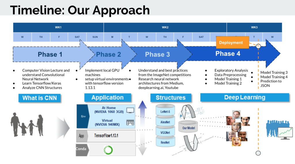
In this blog post, we will explain our approach by studying existing CNN architectures, illustrate our model and results, and give some practical advice for deep learning.
If you need a bit of review on deep learning concepts and CNNs, we’ve compiled some resources that might be helpful.
View our code files on our github accounts (Paul and Jonathan)
Dataset of Images:
We have used dataset provided from our partnering company, MotionFlow, as well as face dataset found from UTKFace. Our dataset comprised more than 23,000 images with labeled age, gender, and ethnicity. Each file name included the true value of age, gender, and ethnicity of the person in the image.
Labels:
The labels of each face image is embedded in the file name, formatted:
[age_gender_race_date&time].jpg
- age: an integer from 0-116
- gender: either 0 (male) or 1 (female)
- race: an integer from 0 to 4, denoting Caucasian, Black, Asian, Indian, and Hispanic
- date&time: format of yyyymmddHHMMSSFFF
Exploratory Analysis
In order to get a better sense of the balance and spread of our set of 23,000 images, we needed to parse the filenames and store them into a dataframe for analysis.
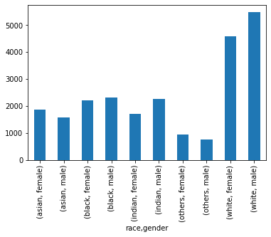
Our dataframe included columns for the file pathway, age, race, and gender. When grouped by race and gender, we found that there are far more images that are labeled as “white male” and “white female” than the other groups. In addition, the differences in count between male and female were relatively similar.
When looking at the histogram for age overall, it’s clear that there are many images of people in their mid-twenties and early thirties. We also made density plots of age after they were grouped by gender and race, which revealed that infants were also proportionally over-represented in the data set.
Knowing that infants aren’t the target audience in practical terms for MotionFlow (ads will most likely not be intended to be read by the infants themselves) and it might be difficult to distinguish features which identify gender and possibly race, we did not include pictures of ages under seven. Next, we made a function that took the continuous values of age and grouped them into age groups, seen below. When coded, age group became an ordinal variable.

Generally, it’s a good idea to balance the dataset across all categories when training a model so that it’s not trained expecting a certain proportion of one category. However, balancing the data across all gender, age, and race categories by undersampling would make the data set too small because there are some combinations of categories with only 8 or 9 pictures.
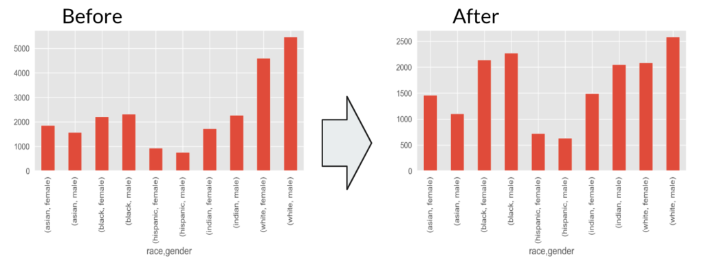
There’s a method called data augmentation, which distorts, rotates, or flips the images to create more samples, but this technique alone on some granular subcategories (like 75+, other, male) would not solve the data size issue. Therefore, we just undersampled the white category by 50 percent at random and saw how our model performed with a somewhat unbalanced data set. Below is the bar plot of counts grouped by race and gender after the white category reduction.
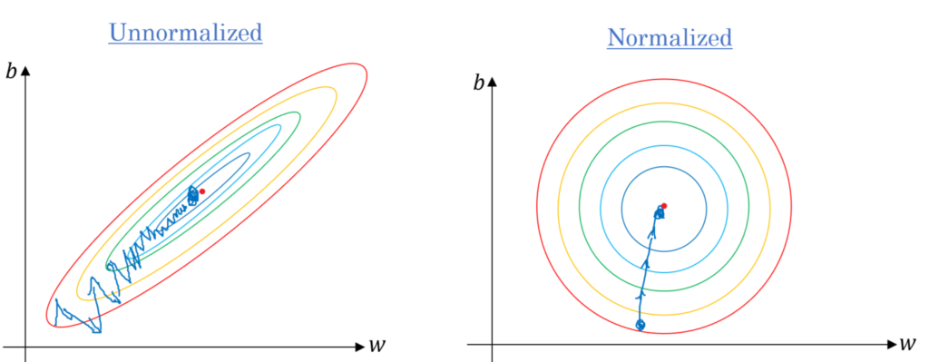
Before we use the JPG pixel values as input values for the CNN model, simple normalization is performed. This is done because we want to ensure equivalent effect on every dimension when doing backpropagation and it also converges much faster from the gradient error.
Model
Before creating our own model, we identified the key benefits and strengths of each structures of architectures which have done well in prior ImageNet competitions (image classification competition) including LeNet-5, AlexNet, VGGNet, and ResNet.
Looking at the architecture of these models, we noticed that we noticed that as accuracy improved these models increased the number of layers and complexity. For our model, we combined the uniform and repetitive convolution layers of VGGNet model with the use of dropouts from AlexNet. As seen below, our model uses 6 convolution cycles, each consisting of a convolution, batch normalization, and max pooling layer, and two dense layers with dropout.
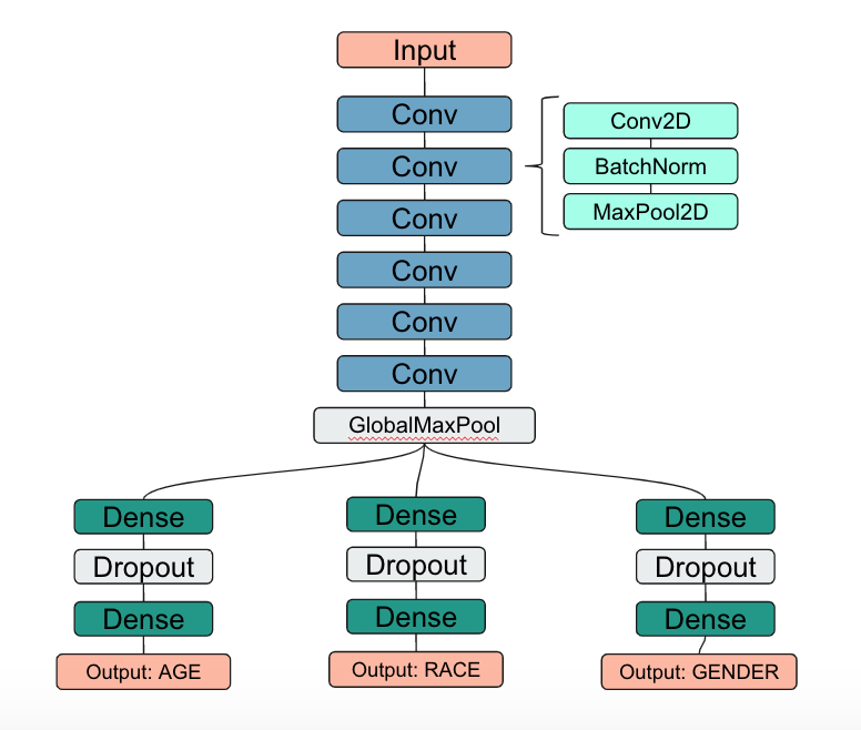
As our data flows through the network of Conv2D layer, the weights and parameters may get too big or too small again. Therefore we set a batch normalization layer in between to normalize our data and converge much faster when training layer.
We used max pooling following the batch normalization to reduce the dimensions of the input volume for the next convolutional layer. Its function is to reduce the amount of parameters and reduce the computational burden of the network.
We tried a few variations of our model using ReLU as our activation function, one using LeakyReLU, and one replacing our convolution layers with a pre-trained AlexNet model with set weights. The results are shown in the following sections.
RESULTS
ReLU with (Conv -> BatchNorm -> MaxPool) * range(3,6)
The first model we tried used the same architecture as shown above, using ReLU as the activation function and the dropout rate was 50 percent. The details of each layer is shown in the image below. There were over one million trainable parameters.
As seen from the output below, the accuracy the race, gender, and age for the validation set was around 70, 90, and 47 percent respectively after 14 epochs.

This was not too bad, but we wanted to see how this could be improved.
LeakyReLU with (Conv -> BatchNorm -> MaxPool) * range(3,6)
Our results using LeakyReLU were slightly better overall, but the accuracy did not continually improve after a handful of epochs like we saw in the previous model. The values of the validation accuracy remained around 76, 92, and 50 percent for race, gender, and age respectively.

Next, we wanted to see how transfer learning could be used to our advantage, using pre-trained weights from an existing model to jumpstart the training process and hopefully improve the accuracy of our model.
Transfer Learning Using ResNet
As seen above in the figure comparing the performance of famous models, ResNet architecture has significantly improved performance. The key to being able to train such a very deep network is to use skip connections. the network will be forced to model f(x) = h(x) – x rather than h(x). This is called residual learning.
We were able to load a pre-trained ResNet model into our own model’s architecture and train our model, only adjusting the weights of our dense layers at the end.

Surprisingly, the ResNet transfer learning model performed quite poorly, only achieving 27, 52, and 11 percent accuracy for the validation set for race, gender, and age respectively.
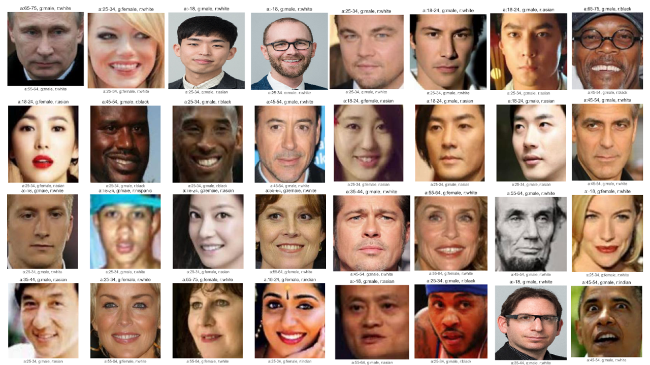
Below is the 32 example outputs as in image format. Prediction is written on top and actual is presented on the bottom.
Conclusion and Next Steps
Our best performing model, using our own CNN architecture and LeakyRelu, achieved 75, 92, and 48 percent accuracy for predicting race, gender, and age respectively. Here are some next steps that would possibly help improve the model’s performance:
- Try other combinations of data transformations, percentage of dropout, activation functions, and see which combinations work well.
- Train three separate models for each type of output.
- Use grayscale images instead of color images.
- Balance the training data set further.
Looking back on our approach, it might have been more appropriate to train three separate models for each of the desired targets. This would have solved some of the data limitation problems when balancing the data set because separating the images by label would have been easier if age, race, and gender were treated independently. Also, it was suggested to us that using grayscale images and further balancing of the dataset would have resulted in a better performance.
Practical Tips
Setting Up Your Environment
TensorFlow updates its versions frequently and often makes code from earlier versions incompatible with the new version. To save yourself headache, set up a different local environment using Anaconda Navigator. For example, if you want to follow along with a YouTube tutorial and they are using version 2.0 but you already installed version 1.13.1, just make a new environment and install TensorFlow 2.0. Here are instructions for how you make a new environment. That way you can switch back and forth between projects and environments without having to use or set up a Docker image.
Training Speed
Training CNNs on image data is notoriously slow. Using Jonathan’s MacBook Pro, each epoch took over an hour. Luckily, Paul had a desktop which used GPUs to train our model in which each epoch was about five minutes. Alternatively, we could have used the cloud computing services of Paperspace or AWS. The price is relatively low, but you still want to use your time wisely and be well-prepared in knowing what versions of the model you want to train.
We hope you have enjoyed reading about our project and learned a bit more about image classification using CNNs. Feel free to leave us comments below or check out our other blog posts by clicking the author links.


