Introduction

For the capstone project, we chose to work on Kaggle’s competition on Grupo Bimbo, forecasting the demand for products from previous sales data. Before delving into the project explanation, it will be good to give some brief information about the global baking industry.

Global Baking Industry

The global baking industry is a US$461 billion industry. The product shares in the industry can be seen in the charft below:

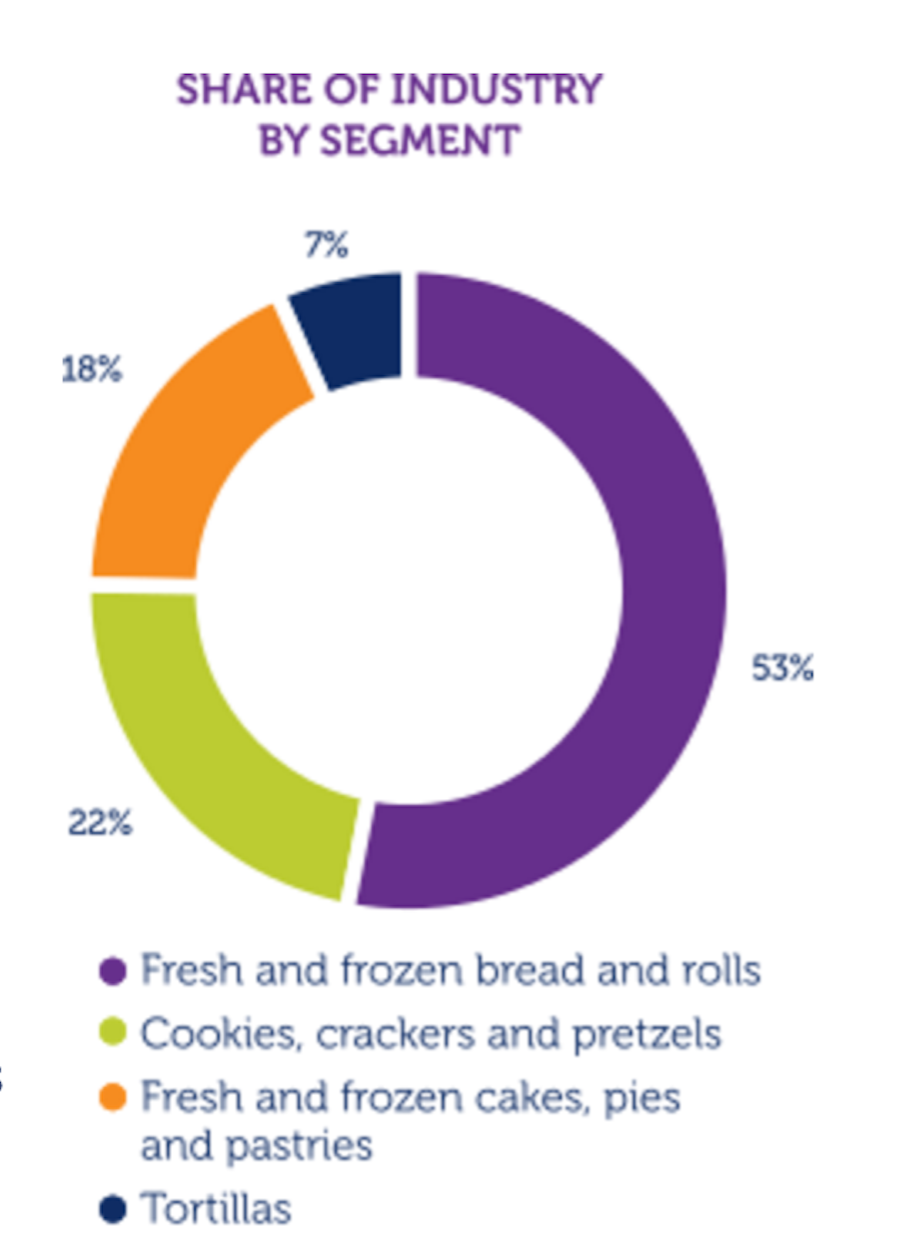
As can be seen from the chart, the largest category with 53% is fresh and frozen bread and bread rolls. Although most of these products are consumed on a daily basis, it is still a growing industry and it is forecast that the annual growth rate over the next five years will be 3%:

The global baking industry is highly competitive with more than 277,000 companies operating worldwide. There are various types of stores providing baked goods, however small bakeries dominate the industry. Besides small bakeries there are also regional family owned bakeries as well as supermarkets and grocery stores with in-store bakeries.

Although it is a competitive industry, there are several major players who compete with the highest market shares. The four major players are Grupo Bimbo, Mondelez International, Yamazaki Baking Company and the Kellogg Company. These four companies account for 10% of the market and Grupo Bimbo is the largest one of these with a 4% market share. The overall market share percentages can be seen from the graph below:

Grupo Bimbo

Grupo Bimbo has over 1 million stores and 45,000 routes in Mexico.  Its annual sales is US$14.1 billion, and it operates in 22 countries. Since the global baking industry is still a growing market, it is important to meet the demands of the customers.  Grupo Bimbo's current inventory calculations are performed by their direct delivery sales employees. They single-handedly predict the forces of supply, demand and hunger based on their personal experiences in each store. For the products which have a shelf life of one week, the error margin is very small regarding inventory planning.

Problem Definition and Datasets

The main goal of the project is to develop a model to accurately forecast inventory demand based on the historical sales data. Five datasets are provided by Kaggle:

• Train.csv (74 million observations)
• Test.csv (7 million observations)
• Cliente_tabla.csv (Client Names)
• Producto_tabla.csv (Product Names)
• Town_state.csv (Town and State information)

Exploratory Analysis

1.Correlation Plot

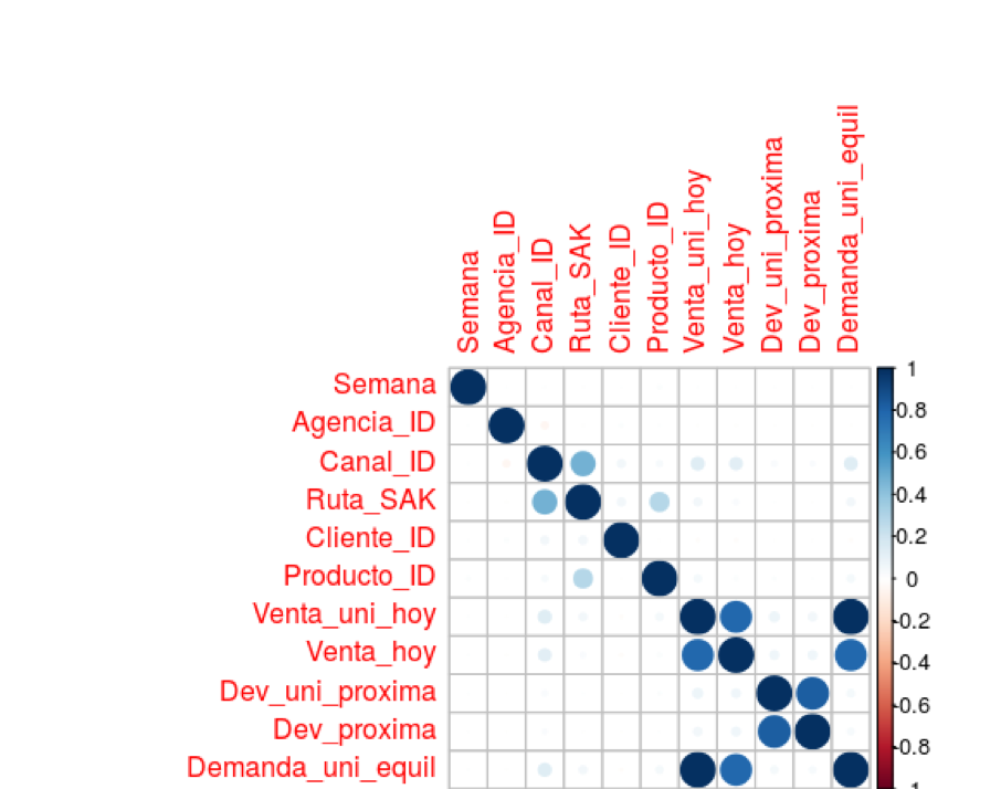
To understand the correlation plot below let us first go through what all the variables are that we were given in the train set. The first variable Semana is the week of the sales/demand. Agencia ID is the Sales Depot. Canal ID is the Channel. Ruta_SAK is the route. Cliente is the client. Producto, is the product. Venta_uni are the units sold. Venta are the sales in pesos. Dev_uni are the number of returns, and the final variable--demand--is what we will be predicting. So out of all the variables we are given, only the last 5 are numeric while the rest are categorical. None of the numeric variables are in the test set of the data, so the problem here is predicting the demand with only 6 categorical features. As we can see in the correlation plot below, demand is correlated highly with sales. We would expect this, as demand is equal to the sales minus the returns. Let us look further into how these numeric features are related to each other and their distributions.

2.Scatter Plot and Distribution

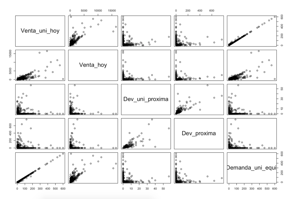
Below are the scatter plots of all the numeric variables provided in the train data. We can see in these charts two things: first, sales almost perfectly match demand, and second, where demand is high returns are low. We see a similar relationship with sales. Low sales mean high returns.

Below are the distributions of the numeric variables which explain why predicting demand will be challenging in this competition. First off, let us look at the distribution of demand. The demand for each client product pair has a minimum of 0 and a maximum of 4777. What makes this so difficult to predict is that the majority of the demand lies between 0 and 6, which means the data has a lot of variance. The standard deviation of demand is 25 even though most of the data is between 0 and 6. As was explained earlier, demand is equal to the sales minus the returns.  This complicates things because almost all of the returns are 0 but the maximum value is up to 500. Both of these factors makes the demand very hard to predict.

3.ProductID / Demand for each week

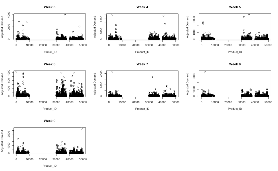
The last bit of exploratory analysis that we did looked at the demand for products each week. We noticed there may be some monthly seasonality in the data. In other words, we found that week 3 looks like week 7 and week 5 looks like week 9. Why this may be important is that the test data are for weeks 10 and 11. This means that week 6 would correspond most closely with one of the test weeks. As can be seen in the graphs below week 6 is the most different from all the other weeks. If this seasonality is correct then that particular week will be very important in predicting the test data.

Implemented Models

The first model we tried was random forests. This model when we tried running it with all of the data kept running into memory issues making it so that the model could not run. After reducing the size of the train data we were using to just one week it was able to run, but as soon as we tried to test any feature engineering the model would never stop running. This continued to happen even after reducing the number of trees and increasing the maximum node. Since the random forest would not run do to the size of the data and the limits of our computational power we decided to try other models.

The next model we tried was Gradient Boosting or GBM. We ran the GBM model with a learning rate of 0.05 and 100 trees, which took 6 hours in total to run. Doing this plus local cross validation we were able to get a rmsle score of 0.64. This however is a much worse score than the public script on Kaggle which takes the medians of demand in an intelligent way. With the bad score and the amount of time it would take to run and test features we decided to try other models.

In the end all of us decided to use xgboost as our model. We did this so we could concentrate on feature engineering and could share both our train sets and have the same baseline for testing our features. We chose xgboost as it both ran quickly so we could test new features and had very good predictive power.

So why xgboost? Xgboost is extreme gradient boosting. It is a more efficient version of GBM, that has both linear model solver and tree learning algorithms. It is fast  as it has the capacity to do parallel computation on a single machine. This makes it 10 times faster than regular gradient boosting. Xgboost can do cross validation, regression, classification, and ranking. Since it can also give feature importance it is a very good model to use in competitions such as Kaggle.

XGBoost Learning Rate and Cross Validation

We cross-validated our results in order to optimize our parameters and test features by using one week out cross fold validation. One of the most important and impactful features that we first implemented was creating a lag of 3 weeks. We did this by creating product client pairs for each week, and then imputing the median of these product client pairs for each similar pairing in the following weeks. So, for example, given week 9, we took the median value of demand from the product client pairs from week 8 and merged them into week 9, creating a feature called Lag1. If the product client pair did not exist in the previous week, it was impute with 0, to indicate that that client had not bought that product in the previous week. By doing this, we reduced our dataset from ~74 million observations to ~40 million observations. Each week that we would have included before week 6 would contain a column of lag with a constant 0 value, because we would not have had data for said week (Given week 5, we would not be able to have a lag of 3 weeks, since we did not have data for week 2), so we removed them from the dataset.

Due to the amount of time it would take to do a full 4 fold, 1 week out cross validation (roughly 2 hours), we decided that it would be more efficient to simply replicate the competition environment via training on weeks 6-8 and testing on week 9. We implemented this validation strategy for the testing of all of our features. Additionally, our 3-week lag features provided the benchmark validation set score through which we determined the effectiveness of the new variables we introduced.

Supply Chain

Features

After attempting our numerous models, we changed strategies and just tried engineering and testing features en masse. We got together and brainstormed about 30 different features to try, divided up the work between the three of us, and got to work. The features and their descriptions that I, Kyle, tried are as follows (With features providing an improvement in bold):

• Weight for a given product
  Thanks to a handy script provided by MetaBaron for the text processing of the spreadsheet including the product names and their associated product ID’s, we were able to easily merge the weight for each product into our training and testing sets.

• Number of pieces for a product
  Similar to the above, we merged the pieces for each product ID into the training and testing sets.

• Weight divided by pieces
  For this feature, we took the weight for each product, and if it was NA, imputed 0, and divided it by the number of pieces (if NA, it was set to 1).

• 3 weeks of lag
  o As mentioned above, this provided the most drastic reduction in rmsle out of any of the other features we tried. We were at about 0.503 rmsle, and this feature alone brought us near 0.48. It is also important to note that since week 11’s 1 week lag feature would be week 10, which we are also predicting on, we used the 2 week lag as both Lag1 and Lag2. Our theory is that once we optimize our predictions for week 10, we will then merge the product client pairs from week 10’s predictions into the Lag1 feature of week 11. Once this is done we will predict on week 11 for our final predictions.

• 5 weeks of lag
  We had also tried 5 weeks of lag, and while giving great results on our cross validation, it had effectively reduced our dataset to only ~20 million rows. We believe that although it provided an improvement on the cross validated predictions between weeks 8 and 9, it did not generalize well to weeks 10 and 11 because of the much smaller amount of training data.

• Brand Name
  Similar to weight and pieces, we were able to merge the brand name of each product into our train and test sets, and tried this feature as both a numeric and categorical feature. Neither improved our score.

• Client Name
  This feature only ended up affecting some 60 thousand of the full ~900 thousand clients. We used the client name spreadsheet provided by Grupo Bimbo and found that many of the client names were street names, prefixed by the store name. An example is shown below with OXXO. What we did to group this is do a find replace on cells containing OXXO, replacing them with simply the store name. We did this similarly with depositos, cafes, hospitals, 7-11’s, etc. For the rest, we gave a client name of “Unknown”. Although this affected a small relative number of clients, it provided a marginal decrease in rmsle.

• Frequency of client product pairs
  We thought that the frequency or number of times a client bought a product in a week would help in differentiating different types of clients. As more frequent purchasers would probably have smaller demand per purchase in a given week.

• Running sum of client product pairs sorted by week
  Next we thought that a running sum of clients buying products would help separate similar clients. Since the data is taken over time you can relate the same number of purchases to each other and possibly predict demand for similar amounts of purchases over weeks. This feature did not end up adding predictive value most likely due to the fact we did not know other than by week when these purchases were made.

• Sum of the lag features
  The idea behind this feature was to sum the median demand for previous weeks. This would differentiate even more clients who had been buying products in past weeks from clients purchasing new products. It also uses one of the features that we found most useful to further differentiate the client product pairs in each week.

• Sum of prior demand
  This feature is the total demand a client product pair had in past weeks and was actually found to be more predictive than just summing the lag features. The reasoning for this feature working is the same as the sum of the lag features: knowing what the client pairs past demand was in each week would help differentiate amounts of demand and help predict future demand for those that had made past purchases.

• Mean prior demand
  This was an attempt to use the mean of the prior demand rather than the sum. it was found to add the exact same amount of predictive value as the sum and therefore was not useful.

• Lag of returns
  This feature has not been tested yet but is a feature that we thought would be a great idea to try. It allows us to use the training data that we do not have access to in the test data, as we have that information for the prior weeks. Once we know how effective this feature is we will update the blog post.

• Town ID
  This feature was added from the Town_State file. After adding this feature we saw that it did not add that much predictive power to our model. as a result, we did not keep the feature.

• Product Count by Town Id
  After adding the town_id feature to our training set we counted the products in each town and added that feature as a new one to our training set. However, our results showed that this feature did not add much to our model so we elected not keep it.

• Client Count by Town Id
  After trying the product count by town we also wanted to try the client count in each town. This feature was the one that we had the least hope for.  However, it turned out to be that this feature helped a lot more than the other features we kept in our model.  We elected to keep the feature in our training set.

• Product Count for each client in each town
  After we saw that client count by town_id added that much to our model, we also wanted to see if adding also the product counts for each client would help.  But this feature did not add predictive power to our model, so we did not keep it.

• Product Count for each client in each route in each town
  We also tried to add the client count in each route as a middle step while we were grouping and aggregating.  However this also did not add that much predictive power so we did not keep this feature.

• Unit price for each product
  By dividing Sales to unit sales we added the unit price of each product as a new feature. However this feature did not that much predictive power to our model.

Feature Importance

The importance of many of the features that we implemented above is shown below through using xgboost’s feature importance plotting. As one can see, the lag features have a large impacted on the predictions of the model. What’s a bit strange is how far down the list the product ID feature is. Also strange, as mentioned above, is how important the town and client count per town features are.

Numeric Added Feature Scatterplot and Distributions

Below is our scatterplot matrix for our different added numeric features against each other and the Demand target variable. As one can see, the lag features seem to be pretty linearly related to the Demand. Again, we see some strangeness with the count variable. There appears to be some sort of pattern there that may make it easier for a decision tree to split on the different values of count.

XGBoost Bagging, Weighted Averaging & Results

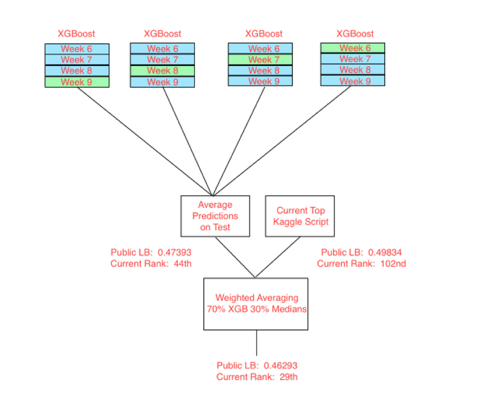
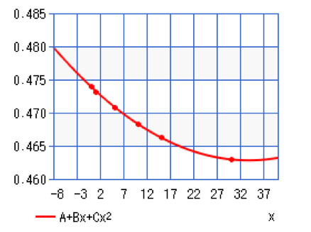
We chose to implement relatively simple ensembling methods to create our current top submission. We turned down the learning rate on our XGBoost from 0.1 to 0.05, and used our validation strategy of training on weeks 6-8 and testing on week 9 to find the optimal number of rounds for this learning rate. We then used 1 week out bagging, training 4 XGBoost models, each time with a different subset of 3 of the 4 weeks of training data. We then took these predictions on weeks 10 and 11 of the test set and averaged them. This gave pretty good results, producing an rmsle of 0.47393. The current top Kaggle script uses the smart merging of previous weeks medians and also does a great job of it, producing an rmsle of 0.49834. This script is quite impressive as it runs in a very short amount of time and does not require the training of any models. We used up almost 2 days worth of submissions plotting the weighted average rmsle scores for 1, 5, 10, and 15 percent top Kaggle script with our corresponding bagged XGBoost predictions. We then fit a polynomial line to this curve and found the minima to be at around 30% Kaggle script, 70% bagged XGBoost predictions. This gave us our current best rmsle score of 0.46293.

Future Steps

For our next steps, we’d really like to try out more features. We still have plenty of ideas left, so at this point it’s just implementing them and finding the ones that work. Some of our ideas currently in the testing pipeline are creating principal components from our numeric features and then using these as additional variables, using monthly clustering.  As we saw in one of our previous graphs, there may be some similarities between weeks 5 and 9, and so on. The strangest week, distribution wise, is week 6, which also give the closest cross validation score to week 10. Another feature to try is biweekly clustering, meaning clustering weeks 6, 8, and 10 together.

As noted above, our current implementation of weighted average is likely overfitting the leaderboard. Although this provides a large decrease in our score, we need to find the most generalizable weighted averaging, and will do so using cross validation. We would also like to do some more sophisticated ensembling once we are able to get some of our other models up and running. Lastly, we would really like to get back to first place.