Banco Santander Retail Customer Satisfaction
Contributed by Sricharan Maddineni, Wendy Yu, Matt Samelson, and Michael Todisco. They are currently in the NYC Data Science Academy 12 week full time Data Science Bootcamp program taking place between January 11th to April 1st, 2016. This post is based on their final capstone project (due on the 12th week of the program).
Banco Santander enlisted the help of the Data Science community in a recently sponsored competition on the Kaggle. The competition objective was to build a predictive model to classify satisfied and dissatisfied customers.
The bank provided both a training and test dataset. The training dataset provided an indicator of client satisfaction. Competition participants were asked to use this set to formulate and tune a model to successfully predict satisfaction of clients in a test dataset for which a satisfaction indicator was not provided.
The training data set consisted of 369 anonymized variables and 76,818 observations.
The Data
Little information was available on the variables. Only the data structure and particular hints in variable names (in Spanish no less) provided insight into how best to pre-process data. Matters were complicated in that it was not immediately clear which variables were categorical and which were continuous. Furthermore, some variables were outright useless in that they consisted of a single value for each observation in the dataset. We observed that the data was largely imbalanced by group. The training set contained approximately 73,000 satisfied customers and approximately 3,000 dissatisfied clients.
Our examination suggested that predictors consisting exclusively of integer values were categorical while the remaining variables were continuous. Utilizing this approach, we separated categorical variables and continuous variables. We identified categorical variables as such and applied centering and standardization processes to continuous variables to remove any unwanted effect in subsequent model fitting due to scaling issues. We also checked categorical variables for zero variance to identify and remove those in which only one value was present for all observations (thereby nullifying their predictive value).
Preprocessing
Pre-processing data is essential to proper model performance in many instances. Many non-parametric models will not perform properly if data is not standardized. Furthermore, unprocessed data sets may have variables with missingness and/or values that have no predictive value (so-called "zero-variance" factors with only one specified level, etc.). Variables with clearly no predictive value are best removed since they consume valuable machine resources when fitting a model. Accordingly, working with missingness and appropriate standardization is an essential first-step to any modeling endeavor.
The Santander data set did not have issues with missingness. Values were specified for all variables. That said, some of the values were meaningless (e.g., "-99999" filler values). The code below depicts the pre-processing steps taken to pre-process the data prior to the commencement of modelling:
The Models
We began by applying high accuracy models to the problem to assess the maximum degree of predictability. Our initial efforts included running boosted tree models and deep learning models.
Xgboost - Sricharan Maddineni
Extreme Gradient boosting is a powerful machine learning algorithm that excels in regression, classification and ranking. Xgboost allows us to achieve a simple and predictive model. Gradient boosting works by creating hundreds of tree models that additively produce one highly predictive model. One deficiency of Xgboost is it can only deal with numeric matrices but this was not an issue in the Santander dataset since all observations were numeric. Xgboost algorithm also appreciates sparse model matrices because observations are denoted as 1’s or 0’s and this simplifies the computational requirements.
The key to xgboost is finding the right parameters by defining the objective function to measure the performance of the model. The equation for the objective function is given as follows:
Obj(Θ)=L(Θ)+Ω(Θ)
where L is the training loss function and Ω is the regularization term.
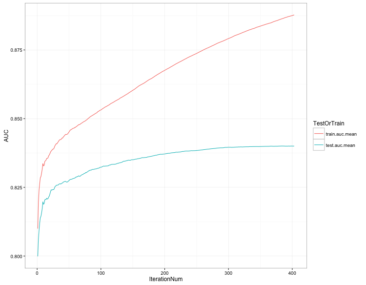
The regularization term controls the model complexity and helps avoid overfitting. For this specific kaggle competition, the AUC was optimized, but it is more common to use the logistic loss.
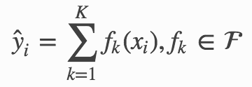
Xgboost is an ensembling tree model where the prediction scores of each individual tree are summed up to get the final score. Additionally, we get CART scores rather than classification values which lend to more interpretability than classifications. Mathematically this is represented as:
where K is the number of trees, F is the set of all CARTS, and f is a function in the functional space F.
The objective to optimize function can therefore be written as:
Creating the sparse model matrix:
Xgboost Model Code:
Making the prediction:
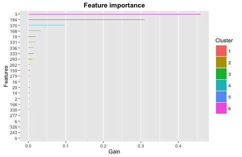
Feature Importance from Xgboost:
GBM Model - Mike Todisco
GBM is a predictive modeling algorithm can be used for both classification and regression. In this instance, we used decision trees as a basis, which is the dominant usage, but GBM can take on other forms such as linear. The model is ‘boosted’ in that it algorithmically combines multiple weak models and it is ‘gradient boosted’ in that it iteratively solves the residuals to improve accuracy. GBM is competitive with other high-end algorithms and has reliable performance. We didn’t have any missing data, but GBM is robust enough to handle NA’s. GBM also makes any scaling or normalizing unnecessary.
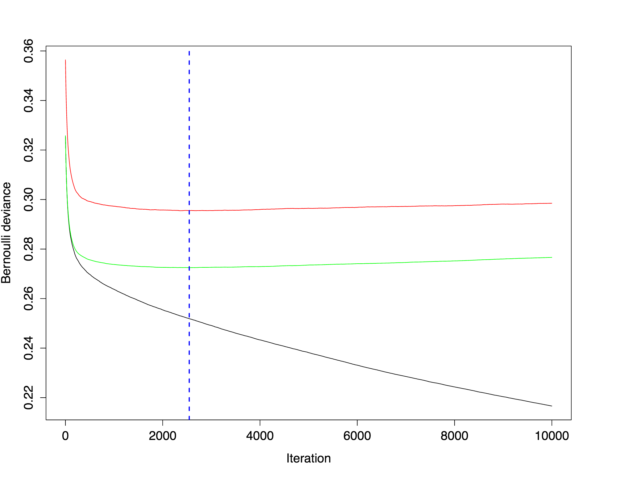
The GBM package has several loss functions that it can run with. We chose to look at two of the loss functions; Bernoulli and Adaboost. Bernoulli is a logistic loss function for 0’s and 1’s. Adaboost is an exponential loss function for 0’s and 1’s.
There are many parameters to tune in the GBM model. Here are a few of the more important ones:
• Number of trees
• Shrinkage – this is also know as the learning rate, dictating how fast/aggressive the algorithm moves across the loss gradient
• Depth - the number of decisions that each tree will evaluate
• Minimum Observations – dictates the number of observations that must be present to yield a terminal node
• Cv.Folds – the number of cross-validations to run
Adaboost Code:
Bernoulli Code:
Random Forest - Matt Samelson
We were able to run a random forest model with optimized parameters in the R Caret package using the train function. This packaging function have some beneficial aspects in that they afford powerful analysis and optimization characteristics not found in underlying packages.
In this instance we elected to utilize the model drawing on the R-based ranger package to generate the forest.
To maximize computational resources we elected to tune three parameters: eta, sample by tree, number of trees per round, and maximum tree depth. The range of parameters can be found in the code displayed below. This was done by means of a grid search in which values were specified for each tuning parameter. The process ran for an astounding 12 hours before yielding the optimal model.
We also employed five-fold cross validation to further optimize the forest construction. Overall model results can be seen in the summary table located at the end of the blog post.
Random Forrest Code:
Neural Net
Random Hyper Parameter Search Random Parameters:
- Activation function to be used in the hidden layers
- The number and size of each hidden layer in the model
- L1 Regularization: constrains the absolute value of the weights and has the net effect of dropping some weights (setting them to zero) from a model to reduce complexity and avoid overfitting.
- L2 Regulation: constrains the sum of the squared weights. This method introduces bias into parameter estimates, but frequently produces substantial gains in modeling as estimate variance is reduced.
- Input Dropout Ratio: A fraction of the features for each training row to be omitted from training in order to improve generalization
- Hidden Dropout Ratios: A fraction of the inputs for each hidden layer to be omitted from training in order to improve generalization.
Neural Net Code:
Model Results
| Model and Parameter | XGBoost | Adaboost | Neural Net | Bernoulli | RF |
|---|---|---|---|---|---|
| AUC | 0.840771 | 0.839205 | 0.821 | 0.820872 | 0.787 |
Model results were highly predictive as expected given the use of non-parametric modeling techniques that emphasize accuracy over interpretation. The project objective was one emphasizing accuracy.
R modeling packages are increasingly improving and providing insight into the construction of complex models. As indicated above under the factor importance chart easily produced after boosted tree modeling in the XGBoost package, 3, 184, 370, and 168 were responsible for a substantial amount of gain in the boosted tree model and therefore have substantial predictive value.
Santander management will hopefully be able to take the results of this endeavor to implement processing that provides both high-level predictive value in identifying dissatisfied clients as well as garnering insight into the factors that drive dissatisfaction.


