What It Took to Score the Top 2% on the Higgs Boson Machine Learning Challenge

Introduction to the Machine Learning Challenge

How do we pit machine learning with physics?

Particle physics is a branch of physics that studies the elementary constituents of matter and radiation, and the interactions between them. Modern particle physics research is focused on subatomic particles that use particle accelerator to break the atoms to detect sub-particles (smaller particles than atom).  The ATLAS detector at CERN's Large Hadron Collider was built to search the mysterious Higgs Boson responsible for generating the masses. The Higgs Boson is named after particle physicist Peter Higgs, who with other five physicists predicted the existence of such a particle in 1964.

On 4 July 2012, the ATLAS and CMS team announced they had each observed a new particle in the mass region around 126 GeV. This particle is consistent with the Higgs Boson predicted by the Standard Model. The production of a Higgs particle is an extremely rare event and it takes years to find this particle. It is a challenge for physicists to analyze such massive data with extremely weak signal.

On May of 2014, the physicists at CERN corroborated with Kaggle to come up with a machine learning competition designed to pit the best of what the technology can bring to the table and predict particle collision events as being the Higgs Boson signal. The challenge was the biggest ever for Kaggle, which attracted 1,785 teams, amounting to 35,772 entries. While the competition has already ended successfully, the Kaggle Higgs Boson Challenge remains one of the few standards by which machine learning specialists can apply and test their skills. One can still submit predictions and Kaggle will be able to score and rank the submission based on how accurate the signal predictions are. It is not an easy task, nor is it for the faint of heart. But in just under two weeks time, with a team of four, we are able to climb the Kaggle Leaderboard ranks and hit the 34th position out of 1,785, placing in the top 2%. This blog serves to document how we accomplished this.

The challenge is to apply machine learning to predict CERN’s simulated particle collision events as either a Higgs Boson signal (s) or background (b) noise. In addition to this main goal and objective, we also wanted learn how to strategize, optimize, and fine-tune models, algorithms, and parameters to achieve the best signal prediction possible, and from there, gain working experience differentiating machine learning theory from actual practice, and develop new skills in model ensembles and stacking techniques.

Success Metrics

In order to track our success and rate of progress, we used the Approximate Median Significance (AMS) score in the Kaggle Private Leaderboard. This is the score by which all submissions are judged on. We measured how good (or bad) we were doing by focusing on improving this score. As we climbed the ranks in the Leaderboard, each 0.01 and 0.001 improvement became exponentially harder and harder to achieve.

That was the success metric we aimed for relentlessly. Improving the AMS score became our obsession for the two weeks we were involved in the challenge. We were shooting for the highest AMS score we can, and aimed to at least be at the Top 25% position placement in the Kaggle Private Leaderboard. By the end of the two weeks. we were not only in the top 25%, we actually placed in the top 2%. It was a very humbling experience to say the least.

The Pipeline Process

We knew from the outset that following the right process was going to be critical. It was clear that the complexity of the challenge and number of variables we were dealing with are many and diverse. We ensured that a process was in place to guide and team tasks towards a focused goal.

So the team followed an Agile methodology. Agile methods normally work wonders for traditional development life cycles in companies big and small, but it has to be adapted to work in a machine learning context where hundreds of data cross-validation cycles are involved. We instituted a lean process to move and fail fast, and perform the wash-rinse-repeat cycle in small iterative cycles. This allowed the team to harvest good results, learn from the bad ones.

We maintained detailed audit trails and logs to understand and review patterns. We started with the basics to get the patterns and trends. We treated data like it's a live entity, understanding it’s health and heartbeat at all times. We got a feel of how the data behaved and reacted to changes, and only attempted to increase complexity of our models and methods only as the prediction accuracy improves. We developed a solid build-create-train-evaluate-predict-score pipeline, and made the iterative process fast, repeatable, and reliable. We then built in feature analysis and engineering to complement the entire development process.

Feature Analysis and Engineering

As a part of feature analysis and engineering, we analyzed missing values and performed various data imputations, addressed correlation and multicollinearity issues, performed the Principal Component Analysis, produced density charts, and understood the -‘phi’ and Jet fields. It was very critical that we maintained a balance in delivering results vs suffering from analysis paralysis. Feature analysis could go on forever and we could glean more and more stories behind each discovery of a significant feature, but it dawned on us from early on that exploratory data analysis (EDA) is only but a small fraction of the effort to serve the ultimate goal. The key on EDA was to discover and test, then explore and exploit.

Technology Stack

A fast machine that can crunch through the model tests and iterations helps, but that's the least of our concerns. Similar to when a photographer takes a great picture, it doesn't mean the camera did it, but it's the method, skills, experience, and process that made it happen. It's no different with machine learning. One can have a very fast machine, but if there is no method to the discipline, everything will just be a random mess.

Python was the preferred language of choice to work on this challenge and was used extensively for all modeling and algorithmic related work, utilizing Numpy, Pandas, Sci-kit Learn & Matplotlib libraries. Python offered us the best performance and scale that we needed for this challenge. R was mainly used for exploratory data analysis (EDA) and plots.

The key Python libraries used are the Scikit Learn suite (Linear_Model.LogisticRegression, svm, DecisionTreeClassifier, Naive_Bayes.GaussianNB), and the Scikit Learn Ensemble (GradientBoostingClassifier, RandomForestClassifier, AdaBoostClassifier). Other special libraries are XGBoost and Neural Network.

Models Used

The following models were used in the Higgs Boson machine learning challenge.

• Naïve Bayes
• Logistic Regression
• Support Vector Machines
• Decision Tree & Extra Trees
• Random Forest
• Gradient Boosting
• AdaBoost & XGBoost
• Neural Networking

Feature Analysis

We start by checking correlation among the features. The correlation plot  indicates a high degree of correlation in terms of number of features and its magnitude.  In the figure below that is indicated by only a small number of crosses for statistically insignificant correlation and dark blue nature of color of correlation .

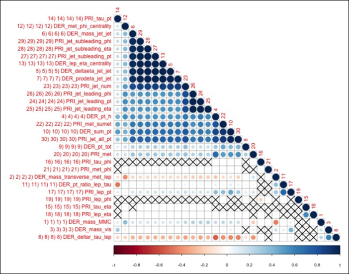
This high degree of correlation motivated us to do a Principal Component Analysis of the data. The scree plot below on the left hand side indicates that a large amount of variance is contained in a small number of principal components than the original number of 30 features. To better visualize this, we plotted the amount of variance explained with number of principal components. We discovered that 90% of variance is driven by only 10 components, and 99 % is driven by 17 components.

So our next challenge was to identify which original features do not have any influence or have very little influence in explaining the data . We start by multiplying the PCA eigenvalues and corresponding PCA eigenvectors and plotted the projections on a heat map. The product calculated in the previous step represents transformed variance along the PCA directions . We then sorted this along the  horizontal axis  by the PCA eigenvalues , starting  with  lowest on the left to the highest on the right . The lower eigenvalue transformed variance  (F 30 - F 17) is zero which is what we would expect from the scree plot above.

We then took another perspective. We sorted the original features along the vertical axis with respect to their contribution to variance in all the transformed variance products with least contribution positioned at the bottom to those that contributed the most on the top .  We summed up the absolute value of the contribution and not just the contribution (as a feature can have positive or negative contribution indicated by red and blue colors). At the end of this process, we are left with features that contribute the least variance displayed at the bottom. It is interesting to note that the plot indicated phi features as having the least contribution - we felt this was one of the more critical information that we used to drive our score up at the latter stages of feature engineering.

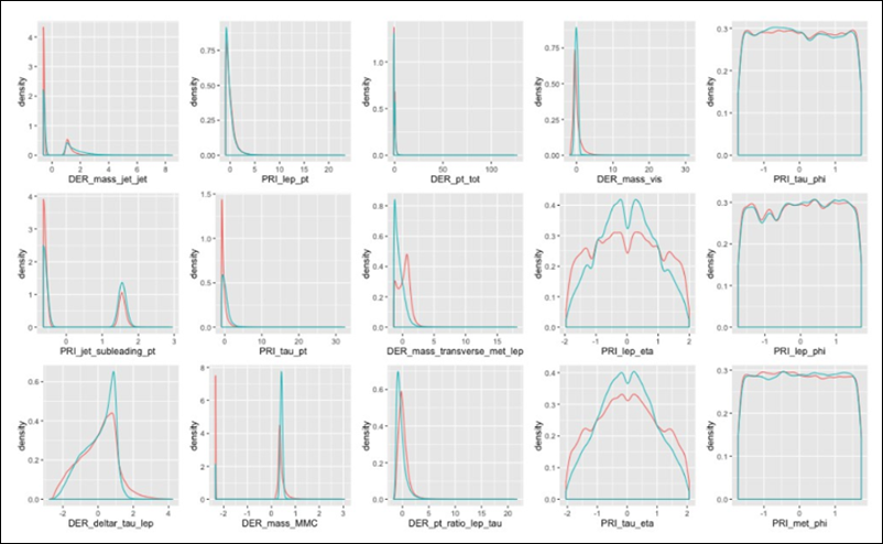
This is further highlighted by the density plots of the features below. The Phi variables on the left showed uniform densities for both the signal and background. indicating that these features are not useful in distinguishing the true signals from the background noise. We can drop these variables without any loss of fidelity against the signal and background information from the original data set.

For a final confirmation, this was also highlighted in the Variable Importance Plot generated by fitting a random forest model to the data. As one can see phi variables as having the least importance in explaining the mean decrease in the accuracy.

One of the peculiar aspect of the data is that it has many values set at -999.0 . From the data description on the Kaggle website, it is stated that those entries are meaningless or cannot be computed and  −999.0 was used to indicate that. One can analyze the amount of -999.0 by replacing them with "NAs" and produce a Missingness plot to explore its frequency and nature. There are 11 columns where values are -999.0 are rampant. Looking at the combinations of features for missing values in the data, six type of data are defined or not defined. In addition, the event corresponds to no jet, 1 jet or more than one jet generation. (2x3).

Overall, we used imputation methods on missing data to test how it would impact the increase or decrease of our AMS score. Imputation methods used were replacing -999 with zeros, mean, median, most frequent existing numbers, or just doing nothing.

Model Training and Cross Validation Results

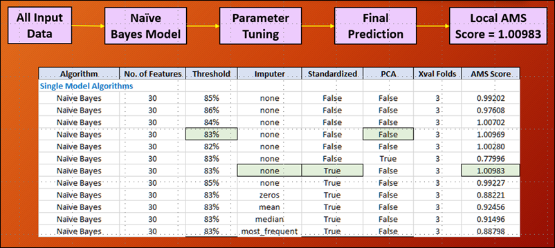
We started off with simple models such as Naïve Bayes and Logistic Regression to predict the class label (Background Noise Vs Signal) for the observations. We leveraged a framework in Python that used the below parameters for tuning the models and calculated the AMS score for each model.

• Number of Features: Total number of features used to train the model
• Threshold: The cut off value for the predicted probability in determining the class label
• Type of Imputation: The methodology used for imputing missing values
• Standardization: Boolean value indicating whether the training data needs to be standardized
• Principal Components: Boolean value indicating whether the Principal components need to be computed for input features
• Cross Validation Folds: Number of splits of the input data used during training and validation of the model

Naive Bayes Model

Using this initial model was needed to get to some idea of what parameters to use to optimize our AMS score. This model provided the benefit pf speed and computing efficiency, albeit at the expense of accuracy, which is perfectly fine for what we needed it to do. We proved out what the EDA theory of missingness showed, which is that the -999 values should be left alone and not be imputed with other values as a substitute. The Naive Bayes model showed this initially, and was proven out even further in other succeeding models used. Numerous tests on the threshold was done and we started narrowing down the range between 80-85% as the background noise.

Logistic Regression Model

We used the logistic regression to confirm the results of the Naive Bayes model, using the same parameters to optimize our AMS score. We made a significant jump in the AMS score just by switching to the logistic regression model, having benefited from the Naive Bayes testing. This will be the ongoing optimization pattern, utilizing results that improve our AMS score and carrying it over to the more sophisticated models.

Neural Network Model

The neural network model is ran with single hidden layer. The reason for choosing single layer is because when tried with two or more hidden layers, the predictive accuracy declined considerably. Neural networks tend to work better for big data sets and in this challenge, having half a million observations is not really considered a big data set. Anything more than one hidden layer would be overkill. The cross validation helped overcome the model over-fitting problem. We tried a lot of feature engineering, like dropping the derived variables, angle variables and grouping the data based on jet value. The model built with the data grouped based on jet value gave the highest AMS score. The following is the detailed log of the neural network model.

Gradient Boosting, Random Forest, and Support Vector Machine (SVM)

As a next step in the testing, Random Forest and Support Vector Machine (SVM) models were evaluated followed by Gradient Boosting. SVM model was run with the Radial kernel using 20% of the training data to ensure the model execution gets completed within a reasonable amount of time. Even with a significantly smaller training data, the model ran for almost 8 hours and had a relatively low AMS score.

The accuracy (AMS ) seemed comparatively better with Random Forest model that built an ensemble of 200 decision trees and averaged the prediction result. The highest jump in the AMS was achieved while using Gradient Boosting model that builds several trees and improves upon the misclassification errors from the previous tree in a sequential manner. This helped the team cross the 3.5 mark in the AMS and gave the first indication that ensemble models provide much better accuracy than single / individual models.

XGBoost

XGBoost implements regularization and parallel processing on top of standard Gradient Boosting that helps in significantly expediting the model fitting and reduces overfitting. XGBoost utilizes OpenMP architecture which can parallelize the code on a multi-threaded CPU automatically. XGBoost has defined a data structure called DMatrix to store and preprocess the data so that the latter iterations run faster. This algorithm allows users to define custom optimization objectives and evaluation criteria adding a whole new dimension to the model and significantly enhances the flexibility.

Dropping the 5-phi Features

We dropped the angle variables based on the insight obtained from the PCA Variable Reduction plot and Variable Importance plot . The AMS score increased to 3.64040. The next least contributing features are the derived variables. So, we dropped the derived variables along with the angle variables and ran the SVM model, the score went down to 0.67110 which is very low. The takeaway is dropping the derived variable is not advisable.

Dropping Features with >70% Missing Data

With the help of Missing Values plot, we found that there are seven features with more than 70% missing values. We dropped them and ran XGBoost model. The outcome was good with scores around 3.4 but did not surpass the best score.

Taking XGBoost Hyperparameters to the Next Level of Tuning

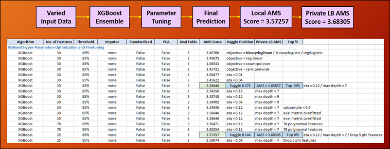
At this stage, we were shooting for AMS score improvements on a 0.01 level. Breaking the 3.6 barrier through XGBoost, we continue find creative ways to optimize this model. This was a crucial step as one of our guiding principals was to optimize the model we worked with to the best of our ability before moving on to the more complex models. So we tried the sharpening and learning rate parameters. Contrary to popular belief that the smaller learning rates are better, it did not work out that way. We were hovering between 0.08 and 0.12 eta rates as the optimal range. We would narrow this down to the most optimal rate at later stages. The maximum depth of the tree was now optimized at 7 for XGBoost, which we consistently used throughout the rest of our tests.

What did kick our score up by a significant amount (going from 15% position to 8%) was when we decided to employ the EDA finding that the (5) phi variables not playing a significant influence to the signal and background data. This was definitely proven out when we dropped these features from the data set. We used this reduced (dropped) set from hereon forward. The dropped set strategy was the result of the EDA discovery work, proving that good EDA utilized at the right time and opportunity can provide significant accuracy to predictions.

At this point, we were very close to breaking the 3.7 AMS score barrier, and we proceeded to employ ensembling and stacking techniques.

Model Ensembling Stacking Tuning

The most rewarding experience of working on this project was the ability to learn and implement the Stacking Machine Learning model.  Stacking is a method that is used to combine the predictive power of multiple classifiers in order to boost the model accuracy significantly. This model utilized three Base classifiers (Level 0) to perform first level prediction in which results were then fed to the meta classifier (Level 1) to combine the individual probabilities and make the final prediction. Several combination of the parameters were tested to check the increase in accuracy for the stacked model as shown in the below screenshot.

This approach kicked us into absolute high gear. We started iterating and optimizing through the various hyperparameters to increase our AMS score. The combination of different ensembles also played a major role. One can not randomly just stack classifiers together and have it improve the AMS score. The guiding principal was to stack as much orthogonality to the classifiers employed to maximize the synergies of those varying approaches.

The few stages of our optimization showed various improvements on our AMS score. The improvements came in excruciating 0.001 increments, but rewarding nevertheless. The results showed a phenomenal overall spike in the AMS metric that helped the team move up through the ranks on the Kaggle private Leaderboard finally ending up at position 34 (out of 1,785 participants), placing finally at the top 2% of the contestants.

Results and Findings

The following are our results and findings based on the Feature engineering and Predictive modeling performed on the Higgs Boson data:

• The analysis helped discover that some variables have certain values that are either meaningless or cannot be computed. These data points are indicated by  −999.0, which is outside the normal range of values for all variables. This is another reason to not impute -999.0.
• Imputation is a not only a bad idea but also incorrect in this scenario  because −999.0 does not indicate a missing value. -999.0 indicates nothing is meant to be there.
• Seven variables are missing more than 70 % of data in the training set. Last variables in PCA feature plots have least influence in their current form.
• Weights and Labels are dependent on each other as shown by Chi square test of dependence. Signal events have low weights and Background events have high weights.
• The Variable Importance plot as well as Principal Components Analysis (PCA) showed that the 5 angle (‘phi’) variables seemed to be the least important of the 30 predictors. Although removal of the above variables did not result in a significant improvement of the AMS score using a single model, it did help increase the score quite a bit for the Ensemble model.
• Ensemble models performed better than single models and stacking the Ensemble models provided the best result in achieving the final AMS score. The final Stacking model consisted of AdaBoost, Gradient Boost, XGBoost as Level 0 classifiers followed by Logistic Regression as Level 1 classifier.
• Stacking several models in the base layer does not always enhance the final result (AMS score). In our testing, three base classifiers (AdaBoost, Gradient Boost and XGBoost) provided almost equivalent results compared to two base classifiers.
• Cross Validation plays a key role in testing the model. Based on our testing, the optimal number of folds for cross validation was determined as 5 since 3 folds seemed to underfit the model while 10 folds seemed to overfit the model.

ROC/AUC Results Curve

Plotting the Receiver Operating Characteristic(ROC) curve helped visualize the performance of the binary classifier in predicting the background noise Vs signal. This graph was plotted for the stacking model that produced the best result in the Kaggle Private Leaderboard. In a ROC curve, the true positive rate (Sensitivity) is plotted as a function of the false positive rate (100-Specificity) for different cut-off points of a parameter.

The area under the ROC curve (AUC) is a measure of how well a parameter can distinguish between two diagnostic groups (background noise Vs signal). Based on this plot, the area under the curve for our best stacking model was found to be ~0.7. This shows that a randomly selected observation from the training data set with the 's'(signal) label has a score larger than that for a randomly chosen observation from the group with the 'b' (Background noise) label    70% of the time.

Lessons learned

This project helped the team learn some invaluable lessons pertaining to Machine Learning, Predictive Modeling and participation in a Data Science challenge.

• An increase in the local AMS score based on the training data does not always translate to an increase in the private Kaggle Leaderboard score due to potential overfitting of the model.
• Combination of  (# of models) x  (# of parameters)  x  (# of features)  is complex and overwhelming. Disciplined process, pipe-lining, and automation are a must.
• SVM is highly computation intensive and the features and parameters need to be carefully selected before the execution of the algorithm. The algorithm runs for several hours even with reduced features and data.
• The maximum number of trees used need not be the same for all the models in a stacked classifier. Increasing the number of trees helped in improving the AMS score only up to a certain threshold. Any further increase in the trees resulted in decreasing the overall AMS score due to potential overfitting.
• As far as insights go, feature engineering (creating new features) did not really work that well – it was not the worth effort. Ensembles and stacking clearly demonstrated significant improvements.
• Hyper-parameters fine-tuning and optimization are very difficult and time consuming because every small change in hyper-parameters could decrease or increase accuracy significantly. A fine line exists balancing across effort vs computing time vs complexity vs accuracy.
• Managing theoretical feature significance to improve prediction accuracy was very challenging in actual practice. Prediction accuracy would have been even more challenging during a real competition due to the absence of the private leaderboard.

Future Work

In terms of what we would have liked to do more of, a few things come to mind. These tasks can be addressed as a part of future scope of enhancements.

• Find better techniques to auto-generate new features to increase prediction accuracy.
• Blend machine learning and physics (or business) models to increase the potential for more accuracy.
• Invest more time and effort to optimize our neural network frameworks.
• Enhance the current Ensemble model by including the Neural Network algorithm (Deep Learning) and test its predictive accuracy. We felt that this area shows tremendous potential.
• Use a Bayesian Optimizer tool to automate pipeline iterations to find best combination of hyper-parameters (given its complexity). A human can not possibly go through the massive amount of hyperparameters manually. Hyperparameter optimizers are designed to use machine learning to improve machine learning, in theory having a machine teaching another machine to excel.

Conclusion

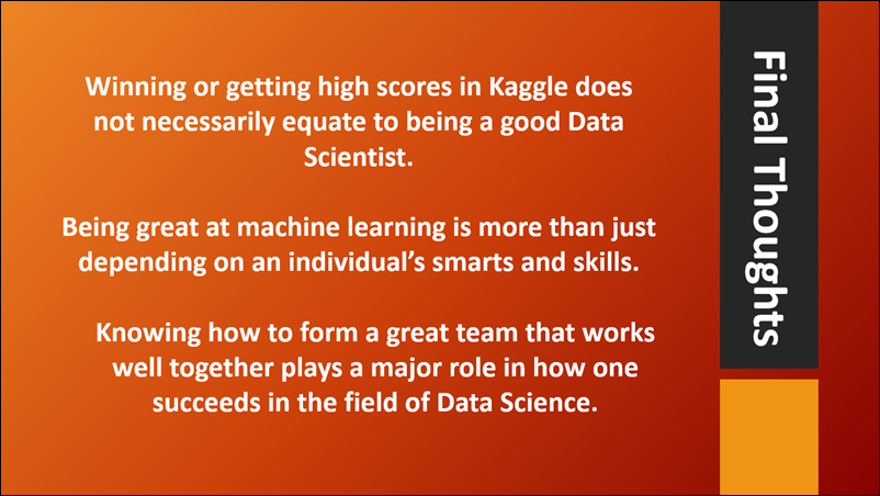
We have met our objectives in this Machine Learning Challenge, being able to apply various models, algorithms, and strategies to achieve relatively good predictions. We have obtained the final private leaderboard score of 3.72254,  ranking 34th out of 1785 participants, positioning us in the Top 2% of the Private Leaderboard. This is a huge accomplishment given that we only had less than 2 weeks to prepare and deliver results on the challenge.

We have a renewed sense of appreciation of what machine learning can do, and also the power behind the complexity. We have learned and developed a lot of new skills from the project, but also realize how much more we still don’t know.