Using Data Algorithms to Predict Housing Prices
The skills the author demoed here can be learned through taking Data Science with Machine Learning bootcamp with NYC Data Science Academy.
Intuitively, which of the four houses in the picture do you think is the most expensive?
Most people will say the blue one on the right, because it is the biggest and the newest. However, you might have a different answer after reading this blog post and discover a more precise approach to predicting prices. In this blog post, we discuss how we use machine learning techniques and data to predict house prices.
The dataset can be found on Kaggle. The dataset is divided into the training and test datasets. In total, there are about 2,600 rows and 79 columns which contain descriptive information on different houses (e.g. number of bedrooms, square feet of the first floor, etc.). The training dataset contains the actual house prices while the test dataset doesn’t.
Dependent Variable
Exhibit 1: Distribution of House Prices
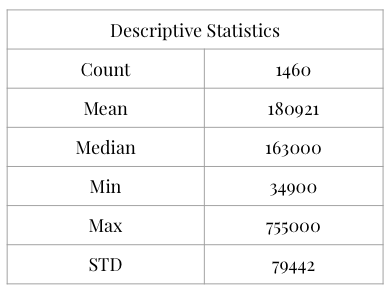
The house prices are right-skewed with a mean and a median around $200,000. Most houses are in the range of 100k to 250k; the high end is around 550k to 750k with a sparse distribution.
Exhibit 2: Descriptive Statistics
Data on Independent Variables
Categorical Variables
Exhibit 3: Overall Quality vs. House Sale Price
Most of the variables in the dataset (51 out of 79) are categorical. They include things like the neighborhood of the house, the overall quality, the house style, etc. The most predictive variables for the sale price are the quality variables. For example, the overall quality turns out to be the strongest predictor for the sale price. Quality on particular aspect of the house, like the pool quality, the garage quality, and the basement quality, also show high correlation with the sale price.
Numeric Variables
Exhibit 4: Above Grade (Ground) Living Area Square Feet vs. House Sale Price
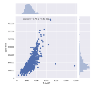
Exhibit 5: Total Feet vs. House Sale Price
The numeric variables in the dataset are mostly the area of the house, including the first-floor area, pool area, number of bedrooms, garage area, etc. Most of the variables show a correlation with the sale price.
Missingness and Imputation
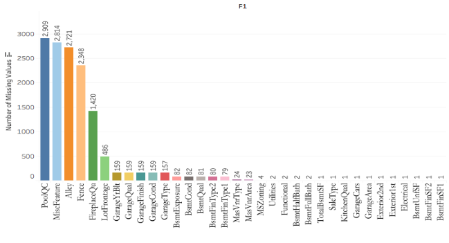
Exhibit 6: Missing Values in Train and Test Datasets
One challenge of this dataset is the missing data. For missing data, such as pool quality and pool area - where a missing value means there is no pool in this house - we replace the missing value with 0 for numeric variables and “None” for categorical variables. However, for missing data that are missing at random, we use other variables to impute the value.
Exhibit 7: Missing Values and Imputation
Feature Engineering
Dealing with a large number of dirty features is always a challenge. This section focuses on the feature engineering (creating and dropping variables) and feature transformation (dummifying variables, removing skewness etc.) tasks.
Drop
Usually it makes sense to delete features that are highly correlated. In our analysis, we found out that GarageYrBlt (year the garage was built) and YrBlt (year the house was built) had a very strong positive correlation of 0.83. In fact, more than 75.8% of these values were exactly the same. Hence, we decided to drop GarageYrBlt since it had many missing values which could be compensated by YrBlt.
Creation
It sometimes makes sense to engineer new features that can help increase the model’s performance. We created the following two new features:
- AgeWhenSold = YrSold - YearBuilt
- YearsSinceRemod = YrSold - YearRemodAdd
Feature Transformation
- We identified 11 ordinal categorical variables where we interpreted that there was some kind of inherent ordering from ‘Excellent’ to ‘Moderate’ to ‘Worst’.
- For the other categorical variables, we used the pandas.get_dummies to get One-Hot Encoding.
- We identified 24 continuous numeric values which has a skew > 0.75 (right-skewed). We used log transformation to get rid of the skewness.
Exhibit 8: Feature Transformation
Regularization
Because we have to work with so many variables, we introduced the use of regularization techniques to address the issue of multicollinearity found in our correlation matrix and the possibility of overfitting using the multiple linear regression model. We address that in the exploratory data analysis section.
The great thing about regularization is that it reduces the model complexity, as it automatically does the feature selection for you. All the regularization models penalize for extra features.
Regularization models include (Lasso, Ridge and Elastic Net). The lasso model will set coefficients to zero, while the ridge model will minimize the coefficients, making some of them very close to zero. Elastic net is a hybrid of both the lasso and ridge model. It groups correlated variables together, and if one of the variables in the group is a strong predictor, then it will include the entire group into the model.
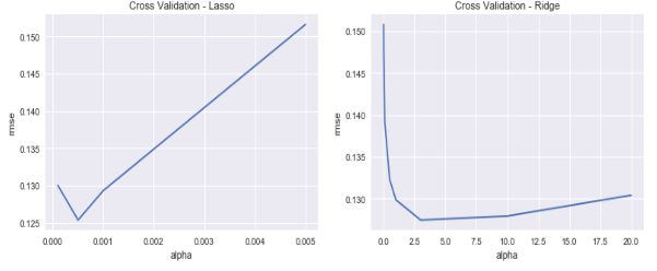
The next step is to tune the hyperparameters of each model through the use of cross-validation.
We choose alpha = .0005 for the Lasso model and alpha = 2.8 for the Ridge model. We choose alpha = .0005 and L1_Ratio = 0.9 for Elastic Net. Because Elastic Net, with a L1_Ratio of 0.9 is very similar to the Lasso model which has a default L1_Ratio of 1, we do not depict it here.
Exhibit 9: Hyperparameters in Lasso and Ridge Regressions
Data on Feature Selection
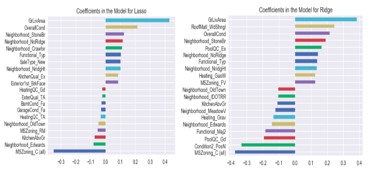
Exhibit 10: Coefficients in Lasso and Ridge Regressions
Lasso Model
Positive coefficients for Sale Price: Above Grade Living Area, Overall Condition and the Neighborhoods (Stone Bridge, North Ridge and Crawford).
Negative coefficients for Sale Price: MS Zoning, Neighborhood Edwards and Above Ground Kitchen.
Ridge Model
Positive coefficients for Sale Price: General Living Area, Roofing Material (Wood Shingle), Overall Condition.
Negative coefficients for Sale Price: The General Zoning requirements, Proximity to Main Road or Railroad and the Pool Quality being in Good condition.
Comparison of our predicted price vs. the actual price on the training data
The two graphs below show how accurate our model prediction is for the sales price vs the actual price. Dots closer to or on the red line show how accurate the model prediction was. There are some outliers that we should investigate as future work on the model.
Exhibit 11: Model Predictions vs. Actual Price
Gradient Boosting Regressor
Gradient Boosting Regressor was one of our best performing algorithms. We first trained gradient boosting machine using the entire set of features (baseline model). We performed cross-validation with parameter tuning using GridSearchCV function from scikit-learn package for Python. Our best model parameters were: learning rate of 0.05, 2,000 estimators and max depth of 3.
We created a relative importance chart to visualize feature importance in gradient boosting. Feature importance scores indicate how useful each feature is in the construction of the boosted decision tree. Above Grade Living Area Square Feet, Kitchen Quality, Total Square Feet of Basement Area, and Size of Garage in Car Capacity were among most valuable features.
Exhibit 12: Relative Importance
PCA + Gradient Boosting Regressor
We then attempted to improve our baseline model performance by reducing the feature dimensionality. High dimensional data can be sparse or spread out, which makes it harder for certain algorithms to train effective models. In general, predictive algorithms benefit from optimal, non-redundant subset of features that improve the rate of training as well as enhance interpretability and generalization.
We managed our machine learning workflows with scikit-learn Pipelines. Scikit-learn Pipeline class allows us to apply a series of data transformations followed by the application of an estimator.
We built several pipelines, each with different estimator (e.g. Gradient Boosting Regressor, Linear Regression, etc.) For Gradient Boosting Machine our pipeline included:
- Feature scaling, using Standard Scaler from scikit-learn package for Python
- Dimensionality reduction, using PCA (retained 150 principal components)
After we completed feature engineering, we had over 200 features and about 1,500 rows in our training set. We decided to keep 150 principal components after examining cumulative percentage of variance chart. 150 components accounted for over 85% of variance of our data. Variance measures how spread out the dataset is.
Exhibit 13: Cumulative Percentage of Variance
Not all tweaks improve results. After we implemented PCA, our cross validation scores did not improve. In fact, our scores deteriorated (cross validation score declined to 0.87 from 0.91 for baseline model). We believe that reducing dimensions caused loss of some important information. PCA not only removed random noise in our data but also some valuable inputs.
PCA + Multivariate Linear Regression
For Multivariate Linear Regression our pipeline included:
- Feature scaling, using Standard Scaler from scikit-learn package for Python
- Dimensionality reduction, using PCA (retained 150 principal components)
Using PCA with Multivariate Linear Regression did not produce good results as well. Our cross validation score decreased as compared to a baseline model (training Multivariate Linear Regression using the entire set of features).
Model Data Comparison
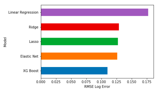
XG Boost model was our best performing model, while multivariate linear regression was our worst performing model. The results were similar among Ridge, Lasso and Elastic Net models.
Exhibit 14: Comparison of Different Models
Using single isolated models gives us a decent result. But usually all real life problems do not have a direct linear or non-linear relationship with the target variable that can be captured alone by a single model. An ensemble of conservative and aggressive, linear and non-linear models best describes the housing price prediction problem.
Stacking and Ensembling
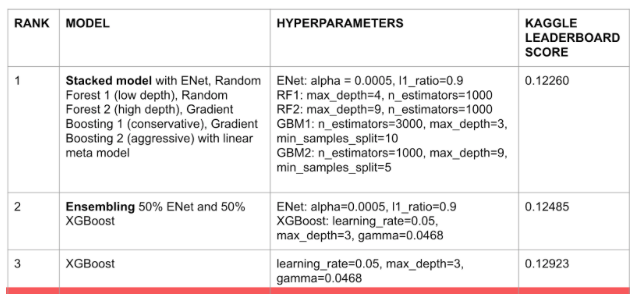
To begin with, we tried a simple ensemble model of XGBoost (non-linear) and ENet (linear) with a 50-50 weightage.
Next, following the standard stacking approach, we stacked different models to see if we could do better. Our stacked model consisted of the linear ENet model, a conservative random forest of short depth, a fully-grown aggressive random forest, a conservative gradient boosting of short depth, and, finally, a fully-grown aggressive gradient boosting model.
The performance has been recorded below:
Exhibit 15: Model Performance
Conclusion
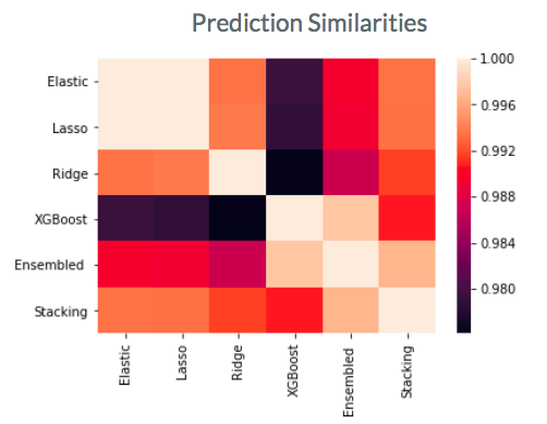
The below correlation heatmap shows our predicted sale prices for some of the models used. We can see that Elastic Net, Lasso and Ridge were very similar in nature, whilst Ensembling and Stacking was also very similar. The one standalone model with distinctly different results was the XGBoost one.
Exhibit 16: Prediction Similarities
Further Exploration
- Explore the correlation between independent variables
- Investigate more feature engineering
- Apply clustering analysis to create new features
- Use different feature selection methods for different models: drop certain features for linear models while keeping most of features for tree-based models


