Data Study on World Health Expenditure and Life Expectancy
The skills we demoed here can be learned through taking Data Science with Machine Learning bootcamp with NYC Data Science Academy.
Introduction
The World Health Organization (WHO) was founded in 1948 by the United Nations. The organization works with countries’ governments and other associations to ameliorate the quality of health for everyone. For the WHO and many other organizations, it is useful to know how to gauge the overall quality of health in a country and more so to know what factors are of the greatest influence. The WHO webpage has data and information on the life expectancy, % GDP expenditure, expenditure per capita, and other indices for each country. One often hears on the news that the US has the highest %GDP expenditure on health in the world, but many countries have better health indices.
Data
Here, I use the data that I scraped from the WHO webpage (http://www.who.int/countries/en/) to show that %GDP expenditure is not the best predictor for better health indices, but that the expenditure per capita has a stronger relationship with life expectancy. A resulting linear model can function as a guide to how much life expectancy can be affected given certain changes in expenditure per capita.
Male Life Expectancy and the Measures of Expenditure
By looking at a plot of the two measures of expenditure considered here in Figure 2, we see that expenditure per capita has a much stronger relationship with male life expectancy then does % of GDP expenditure. Actually, expenditure per capita seems to grow exponentially with male life expectancy.
Linear Model
This exponential relationship between expenditure per capita and male life expectancy can be exploited to create a linear model. In this model, we ask the question “how does male life expectancy change with the natural log of the expenditure per capita”.
The resulting fit of the linear model to the data from the WHO website is shown in Figure 3. The intercept and slope coefficients for the model are β0= 38.916(years) and β1= 4.657(years/log($)). The p-values for the two coefficients are much less than 0.05, implying that both values are significant. The slope value β1 shows a positive relationship between the two variables and indicates how much the male life expectancy changes with a change in the log of the expenditure per capita.
Findings
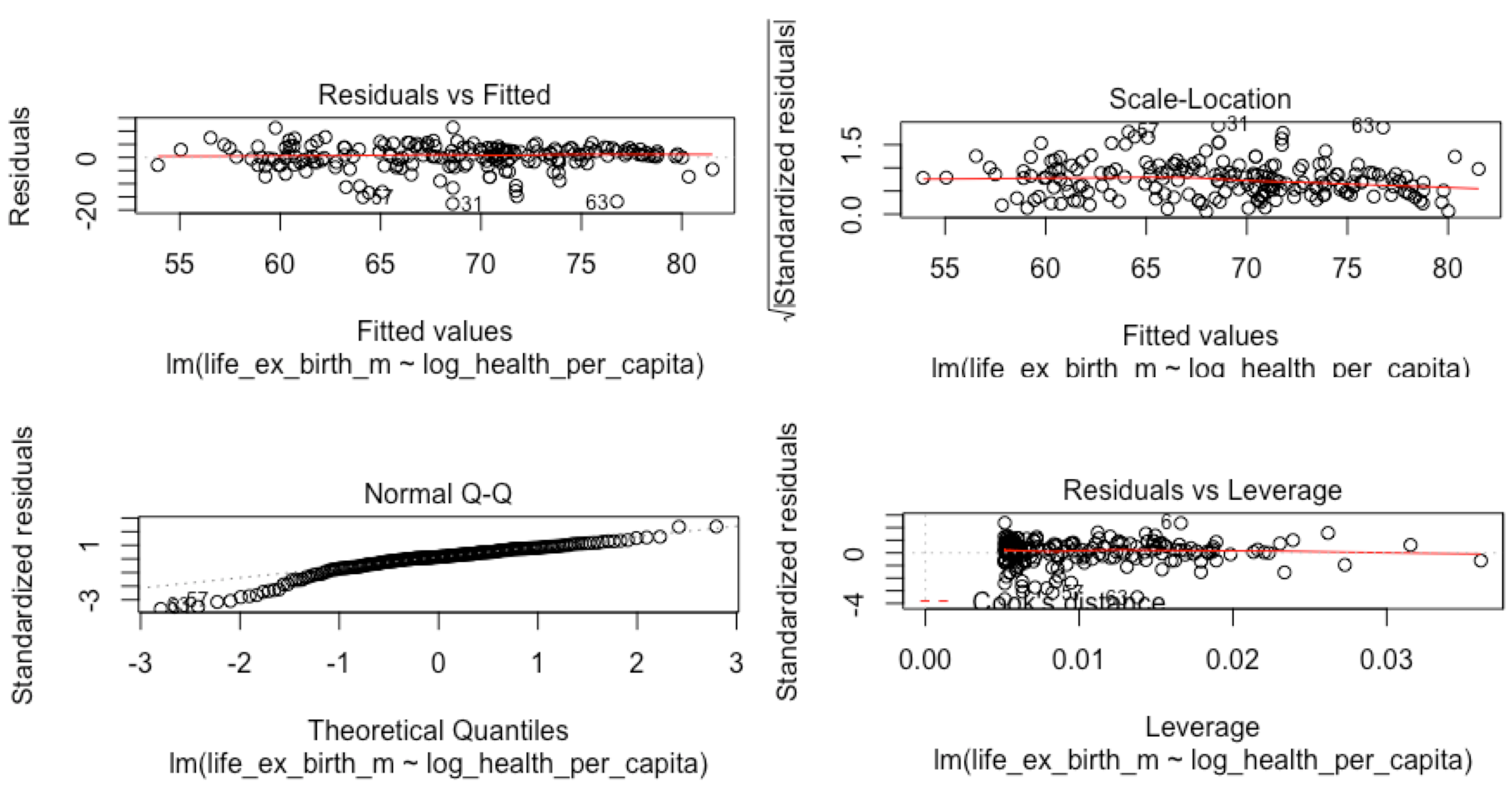
Although it seems that the model in Figure 3 forms a good description of the data, a check of whether the assumptions for forming a linear model are met is warranted. Figure 4 shows some of the diagnostics used to validate our linear model in Figure 3. The positive diagnostics are:
- the residuals vs. fitted curve shows a flat and linear line
- the scale vs. location plot shows that different regions of the fitted values have similar variance
- the residual vs. leverage plot shows that there are no points that are influential (both outliers and have high leverage), and none of the points fall close to the Cook’s 0.5 or 1.0 lines.
The only possible drawback for this model is found in the normal Q-Q plot. While the plot shows that for most of the quantiles the relationship is linear, at the lower quantiles the points deviate slightly from linearity, indicating that the distribution here may be skewed and not normal in form.
It is possible that a different relationship between expenditure per capita and male life expectancy, other than the log(expenditure per capita), may help with some of the problems in the normality of the lower quantiles. To this end a Box-Cox transformation may be performed to find a different linear relationship. However, considering most of the diagnostics, the present model shown in Figure 3 is a good linear model and directly relates expenditure per capita to male life expectancy. The results here show it may be more prudent to discuss health indices with respect to the expenditure per capita in a given country instead of the % of GDP expenditure.


