Kaggle Challenge Top 16%: What We Learned
Introduction
In this article, we outline an approach to feature selection and engineering and machine learning modeling that enabled us to score the top 16% in the Kaggle house price prediction competition.
The Dataset and Competition
The Ames Housing Dataset, consisting of 2930 observations of residential properties sold between 2006-2010 in Ames, Iowa, was compiled by Dean de Cock in 2011.
A total of 80 predictors was part of these dataset:
- 23 nominal
- 23 ordinal
- 14 discrete
- 20 continuous
In 2016, Kaggle opened a housing price prediction competition, utilizing this dataset. Participants were provided with a training set and test set--consisting of 1460 and 1459 observations, respectively--and requested to submit sale price predictions on the test set. Submissions are evaluated based upon root-means-squared error (RMSE) between the logarithm of the predicted sale price and the logarithm of the actual price on ca. 50% of the test data. As such, the lower the RMSE, the higher the ranking on the competition leaderboard.
Exploratory Data Analysis (EDA)
In this section, the data preprocessing, data analysis, feature selection, and feature engineering phases of the project are discussed.
Outliers
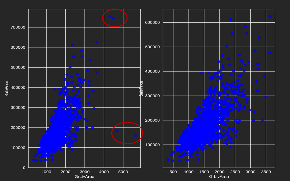
As is indicated in the figures below, 12 outlier observations were removed from the training set after performing simple linear regression on an engineered variable with strong correlation to the response variable (SalePrice):
Response Variable
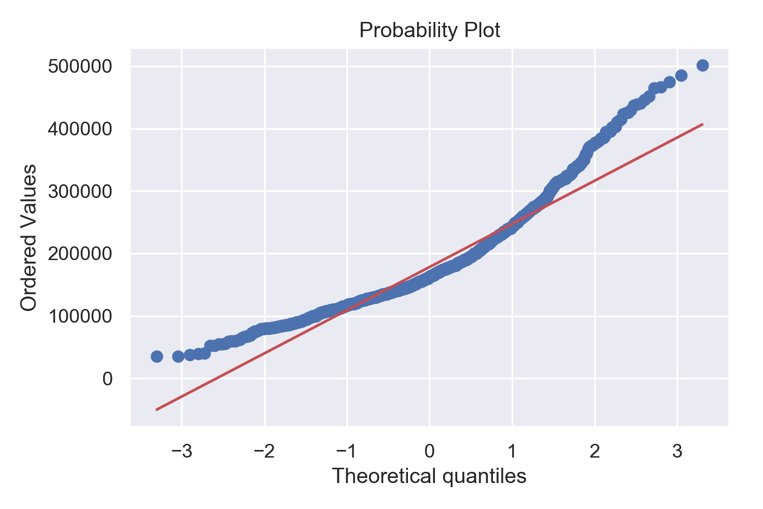
Given that the response variable demonstrates skewness, and that the RMSE for Kaggle submissions is calculated based upon the log predicted price, a log transform was applied to the SalePrice feature in the training set. As a result, the distribution is (sufficiently) normalized:



Correlation Levels
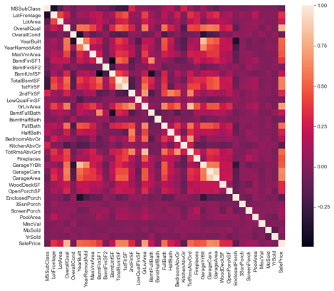
The following heat map visualization indicates levels of correlation between continuous features and the response variable, SalePrice.
Missing Values and Imputation
A significant number of columns contained missing values. However, the reasons for and impact, impact, and type of missingness (missing completely at random, missing at random, and missing not at random) varied.
Fill NAs with mode
- Electrical
- MSZoning
- Utilities
- Exterior1st
- Exterior2nd
- SaleType
Fill NAs with 0
- MasVnrArea
- LotFrontage
- BsmtFullBath
- BsmtHalfBath
Fill NAs with ‘None’
- MasVnrType
- PoolQC
- Fence
- MiscFeature
- GarageType
Feature Engineering
Extract Information from ‘HouseStyle’ and ‘MSSubClass’
MSSubClass: Identifies the type of dwelling involved in the sale
- 20 1-STORY 1946 & NEWER ALL STYLES
- 30 1-STORY 1945 & OLDER
- 75 2-1/2 STORY ALL AGES
- 120 1-STORY PUD (Planned Unit Development) - 1946 &
HouseStyle: Style of dwelling
- 1Story One story
- 1.5Fin One and one-half story: 2nd level finished
- 1.5Unf One and one-half story: 2nd level unfinished
From these two columns, we created new variables in the dataset: Floor, PUD, SFoyer, SLvl, Finish.
Combine Existing Features
- TotalPorchSF = OpenPorchSF + EnclosedPorch + 3SsnPorch + ScreenPorch
- TotalBath = FullBath + 0.5 * HalfBath + BsmtFullBath + 0.5 * BsmtHalfBath
- GarageAge = YrSold - GarageYrBlt
- HouseAge = YrSold - YearRemodAdd
- GarageQuality = (GarageQual + GarageCond)/2
Add New Features
- Added Interest Rates from 2006 to 2010 and concatenated with the sale year and month. (Dataset Link)
- House Price Index in Ames, IA: Average price changes in repeat sales or refinancings on the same properties. (Dataset Link)
- Added School District: One high school, five elementary schools, and one middle school for each row of data.
Final Preparations for Modeling
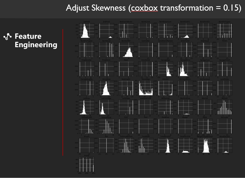
We adjusted the skewness of variable greater than 0.85 with a cox-box transformations of 0.15 and created two versions of the datasets: one in which nominal categorical variables were one-hot encoded for linear regression models, and one lacking one-hot encoding for tree-based models.
Machine Learning Modeling
We first decided to test individual models' performances on Kaggle then pick the best performing models and stack them together.
Step 1: Testing Individual Models
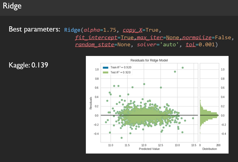
Here are a few example of residual plots for our models:



Step 2: Manual Weight Stacking
Weights:
- XGB = 0.25,
- ElasticNet = 0.2,
- Gradient Boost = 0.2,
- LASSO = 0.15,
- Ridge = 0.1,
- Random Forest = 0.1
Kaggle score: 0.126
Step 3: Further Hyperparameters Tuning and Voting Regressor
We decided to try randomizedSearchCV on our hyperparameter from better tuning. We re-tuned my parameter for each model, and then we did a voting regressor to find the optimal stacking.
Weights:
- XGB = 0.233,
- ElasticNet = 0.1831,
- Gradient Boost = 0.142,
- Lasso = 0.1765,
- Ridge = 0.1533,
- Random Forest = 0.112
Kaggle score: 0.11747
Final Results: Kaggle Submission
The best obtained Kaggle score was an RMSE of 0.11748. This corresponds to the top 16.6% of submissions to date.
![]()
Finally, we have met our objective in this Machine Learning Challenge, being able to apply various models, and strategies to achieve relatively good predictions. However, winning or getting high scores in Kaggle does not necessarily equate to being a good Data Scientist. Knowing how to form a great team that works well together plays the most dominant role in how one succeeds in the field of Data Science.
What We Learn As A Team:
- Occam's Razor: One should not make more assumptions than the minimum needed. In Data Science, it is highly preferred to have interpretable models to get a thorough understanding of the underlying problem.
- Rule of Simplicity: The simplicity vs complexity trade-off is typically evaluated by both the decision maker in collaboration with the data scientist. It is important to note that although simplicity is an important focus, it should not become a blind obsession. As a team, we learn that we should focus on solutions rather than techniques.
- Solution oriented, not technique oriented: Corporate governance and management oversight is key to the success of analytics!
Future Work
- Looking into different imputation methods and see how they influence the predictability.
- Blend machine learning and real life physics models to increase the potential for more accuracy.
- Add extra outside data-set and run it toward our model again.
- Use a Bayesian Optimizer tool to automate pipeline iterations to find best combination of hyper-parameters.
- Spend more time interpreting the result
Project GitHub Repository || Jayce Jiang LinkedIn Profile


