Data Study on Option Pricing
The skills we demoed here can be learned through taking Data Science with Machine Learning bootcamp with NYC Data Science Academy.
Contributed by Ruonan Ding. She is currently in the NYC Data Science Academy 12 week full time Data Science Bootcamp program taking place between April 11th to July 1st, 2016. This post is based on her third class project - Web Scraping (due on the 6th week of the program)
Goal:
This exercise illustrates the Option Pricing techniques of Binomial Tree option pricing and Monte Carlo simulated method in pricing. Black-Scholes model is not demonstrated here since it is a data and formula based method that doesn't give flexibility of constructing exotic options.
The example is Russell 2000 Index. The data was scraped from yahoo .finance from 12/1/2015 to 5/2016 using Scrapy. The option to price in the example is a call option strike price at 980 and exercise date on 6/17/2016.
Data
Price of the underlying index:
This is the price of the underlying index Russell2000 over the past 6 months.
and the daily volatility is graphed as below. This shows the magnitude of changes bouncing up and down daily of the Russell 2000 index.
Option Pricing Assumption:
- exerciseDate : 6/17/2016
- exercisePrice : 980
- timeToExpiry : 29 days
- underlyingPrice : 1094.76
- expectedVol : 0.1486
- riskFreeRate : 0.03
Pricing Method 1: Binomial Tree
Binomial Tree is essentially replicate the payoff of the derivative with the stock and a risk-free bond. We define the risk-neutral probability of the stock price going up as follows, assuming a Cox-Ross-Rubinstein tree:
- u = e^(σ√h)
- d = e^(−σ√h)
- p =e^(r−δ)h − d/(u − d)
- C0 = e−rh[pCu − (1 − p)Cd
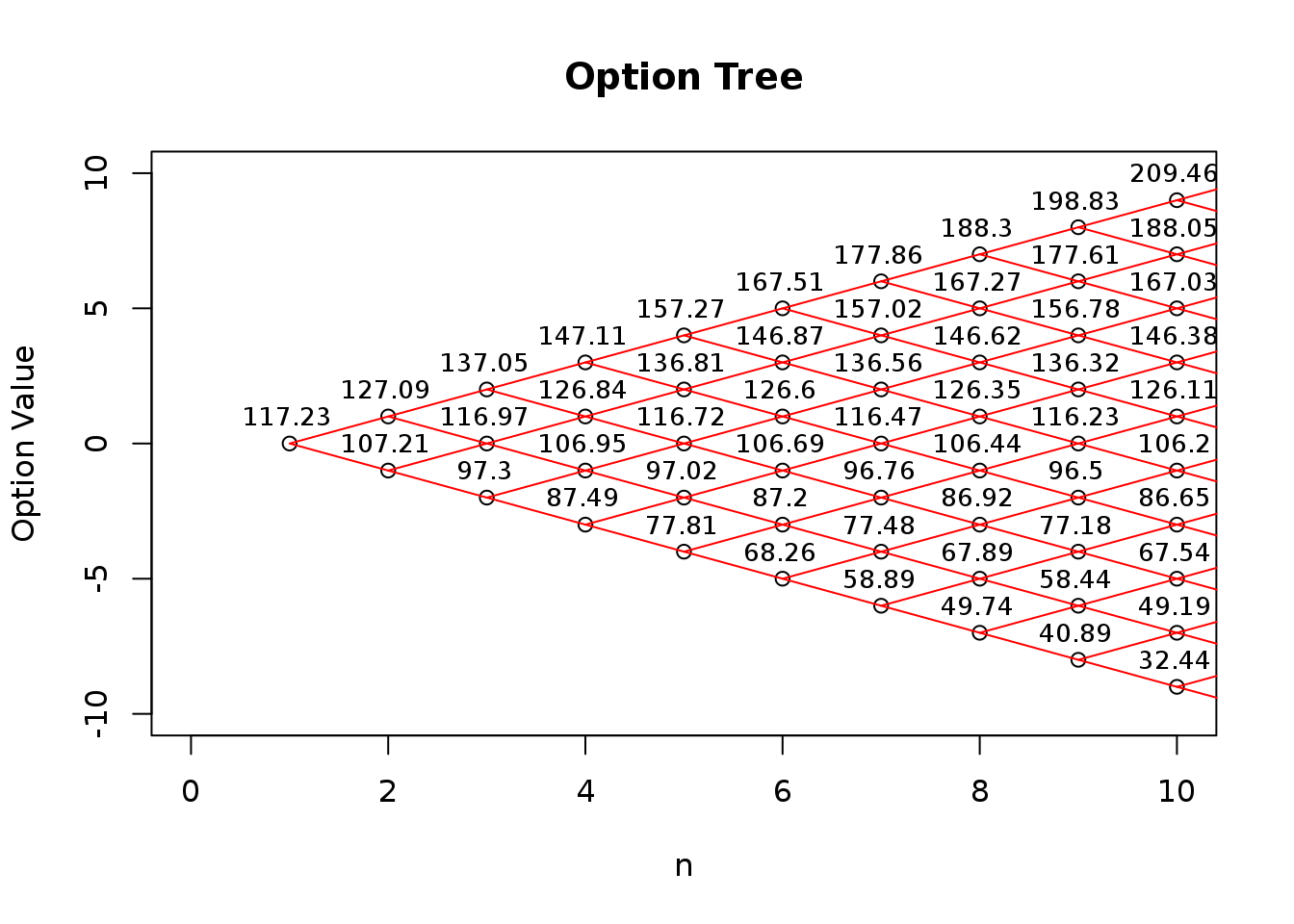
Below is the construction of the option pricing tree of 29 days. Given the scale of the graph, only the first 10 days option prices have been shown here on the graph. However the same method applies across the entire holding period. Payoffs were being calculated at each node on the tree here according to the probability and volatility of going up and down. The final priced option at the root, which is today, is 117.23.
 Pricing Method 2: Monte Carlo Simulation
The way we’re going to simulate stocks is by taking advantage of the lognormality of stock prices. We’ll use the following method: start with iid uniform numbers u1, u2, …, un, calculate z’s where zi = N^(-1)(u1), convert these to N(µ, σ2) random variables by letting r1 = µ + σz1.
To simulate a single stock price the following formula can be used:
S(T) = S(0)e(α−δ−σ^2)T +σ√T z
Below is 20 out of 10000 simulated stock price at the time of expiring## [1] 1066.7280 1163.9929 1062.4881 974.6737 1117.2668 1131.5114 1165.4857
## [8] 1086.3615 1147.9924 1090.1666 1124.2775 1181.3669 1083.9656 1069.3006
## [15] 1174.8100 1104.7534 1053.5856 1077.2294 1065.0571 1024.4855 1084.3327
## [22] 1133.4881 1103.6716 1118.3079 1064.6554 1094.3255 1150.0903 1094.5243
## [29] 1049.9021 1139.1014 1121.6219Based is the simulated payoff given the stock price we just simulated at expiring.## [1] 86.72802 183.99287 82.48810 0.00000 137.26685 151.51141 185.48574 ## [8] 106.36153 167.99241 110.16656 144.27751 201.36691 103.96565 89.30063 ## [15] 194.81002 124.75345 73.58560 97.22937 85.05710 44.48549 104.33266 ## [22] 153.48814 123.67161 138.30794 84.65539 114.32553 170.09025 114.52428 ## [29] 69.90208 159.10135 141.62188
Option price is average the simulated payoff at expiring discounted back to current, which is $118.0301


