Big Data Analytics: from Impressions to Clicks
Post Content:
- About the Project
- Data Exploration Steps
- Data Exploration: Duplication in Clicks Dataset
- Merging Impressions & Clicks for Modeling
- Predictors of Clicks & Feature Engineering
- Exploring Bivariate Relationships with Clicks
- Addressing Imbalanced Classes on the Target Variable
- Predicting Clicks: Logistic Regression
- Predicting Clicks: Random Forest
- Predicting Clicks: Feature Importances
- Future Research Directions
Project Background & Objectives:
We were very excited about this project because it gave us an opportunity to finally deal with the "BIG DATA"!
Inputs we worked with:
A digital company involved with placing bids for clients' online ads provided us with the following:
- three datasets on an Amazon Simple Storage Service (S3), each representing a sample of September 2016...
- bid requests they placed
- impressions from those bid requests, and
- clicks for those impressions
Objectives:
- Explore the datasets and report anything noteworthy
- In the Impressions dataset: identify potential predictors of clicks and engineer features for predictive modeling
- Predict Clicks vs. non-clicks using Machine Learning algorithms in Apache Spark (Python)
Tools at our disposal:
- Data storage with AWS: S3
- Data processing: Spark based on a 16-core AWS cluster)
- Databricks platform
Project Workflow:
Data Exploration Steps:
- Working through a sample of data locally, on our laptops, we sought to understand each variable within the three datasets and how those datasets related to each other.
- Later, we repeated this step using Spark on the cluster.
- We looked at:
- The meaning of each variable
- How likely each variable was to be a predictor of clicks
- Percent of missing values on each variable
- For categorical variables: Number of levels and their incidences
- For numeric variables: distribution
- Relationship between each potential predictor and clicks (vs. non-clicks)
We found duplications in Clicks dataset: Certain ads were clicked on multiple times by the same user!
- Found no unique row ID in Clicks nor in the Impressions dataset
- Our client company informed us that a combination of ‘impId’ and ‘dimensions’ should provide a unique row identifier
- However, we still found duplicate combinations, i.e., multiple clicks per impression on a single occasion (i.e., one impression for a specific user)
- Most duplicates were due to multiple clicks happening within a very short amount of time (even a few seconds)
We defined as “abnormal” 5 or more clicks per impression occasion and take a look at those cases
122 impId/dimensions combinations has more than 5 clicks per impression (0.025% of all impId/dimensions combinations in Clicks)
We took a closer look at them...
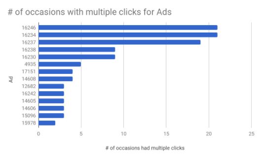
Of 27 ads with multiple clicks per impression, 14 had multiple clicks on more than 1 occasion.
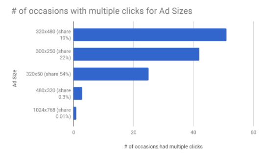
Ad sizes 320x480 & 300x250 were most likely to had multiple clicks on many occasions - despite their lower share in Clicks data (share = proportion of rows for a given Ad size).
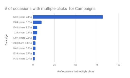
Of 15 campaigns with multiple clicks per impression, 9 had multiple clicks on more than 1 occasion - not in line with their share.
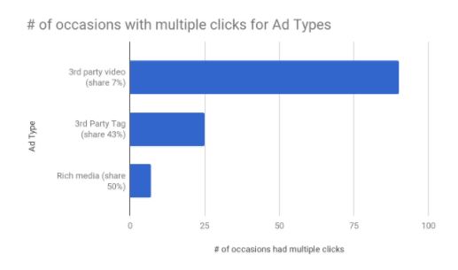
3rd party videos were much more likely to have multiple clicks per impression, despite their low share.
Toyota.com, for example, had experienced much larger number of multiple clicks per impressions than its overall share would dictate.
Merging Impressions & Clicks for Modeling
Merging Steps:
- Impressions containing predictors, we needed to add click/no click information from Clicks → we created a new column click_status in Clicks, filled with 1s
- We de-duplicated both Impressions (based on dimensions and auctionId) and Clicks (based on dimensions and impId) and created a new column dim_id in both data sets (based on dimensions and auctionId/impId)
- We merged Impressions and Clicks based on dim_id and filled all NAs in click_status with zeros
Now, our new column click_status in Impressions could be used as a target variable for predictions (1 = click, 0 = no click)
Dropping Rows:
- Originally, our Impressions dataset had ~300 million rows
- After de-duplication based on Dimensions and AuctionId, Impressions had ~294 million rows
- We decided to exclude non-US countries; after they were dropped, Impressions had ~266 million rows
- Upon merging Impressions & Clicks, we discovered that some ads had no clicks at all! Apparently, it was because the dataset we received from our client was a sample. We decided to drop the ads without any clicks. After dropping all records for the ads without clicks, Impressions had ~ 70 million rows
- We also dropped ~2% of rows with unknown location and ended up with ~ 69 million rows
Predictors of Clicks and Feature Engineering
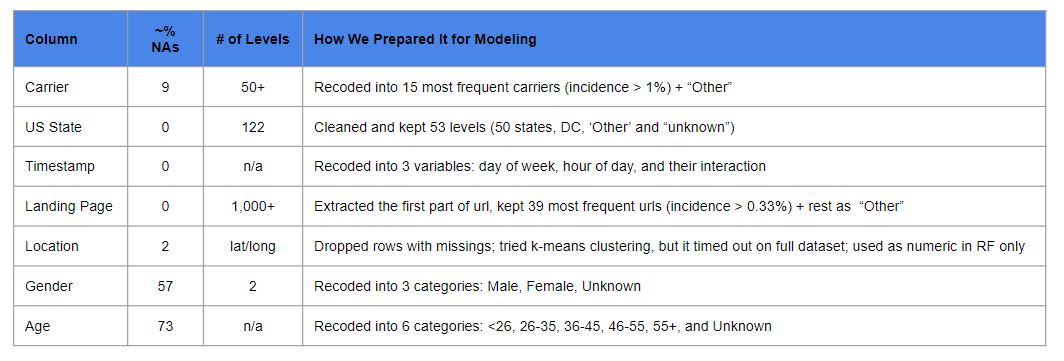
The table below shows columns we decided to use as predictors of clicks, % of Missing values (NAs) for each of them, # of levels and how we recoded the columns for modeling.
The following columns had no missing values and were used as is: Ad Size (7 levels), Ad Type (3 levels), Device Type (4 levels), Exchange (4 levels), Venue Type (4 levels), and Target Group (1,200+ levels).
Exploring Bivariate Relationships with Clicks
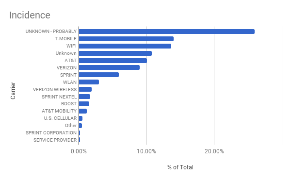
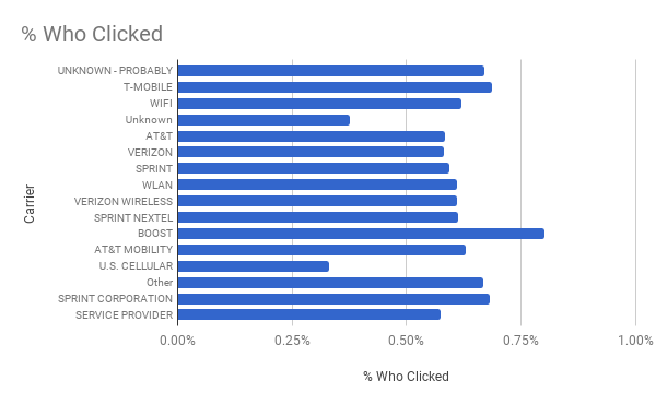
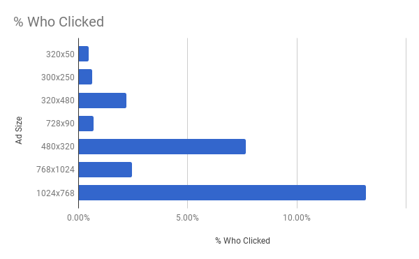
Several graphs below show the results of our exploratory data analysis devoted to the bivariate relationship between predictors and clicks. For each predictor, we first show its levels and their incidences and then % of clicks for each level.
Incidence & Relationship with Clicks: Gender
Looks like Males are more frequent ‘clickers’.
Incidence & Relationship with Clicks: Carrier
Clicks seem to be somewhat less frequent for ‘US Cellular” and some minor carriers (fall under “unknown”)
Incidence and Relationships with Clicks: Ad Size
Larger ads are clicked on relatively more frequently.
Incidence Type and Relationship with Clicks: Ad Type
3rd Party Video ads are clicked on relatively more frequently.
Incidence Type and Relationship with Clicks: Device Type
PC users seem to be less generous with their clicks.
Incidence Type and Relationship with Clicks: Exchange
Ads purchased on Rubicon seem to attract fewer clicks.
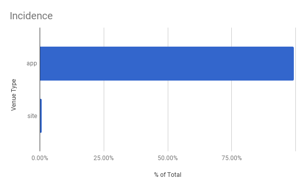
Incidence Type and Relationship with Clicks: Venue Type
Ads shown on apps seem to attract more clicks than those shown on websites.
Incidence Type and Relationship with Clicks: State
Relative frequency of clicks is different from state to state.
Incidence Type and Relationship with Clicks: URL
Relative frequency of clicks is different from url to url.
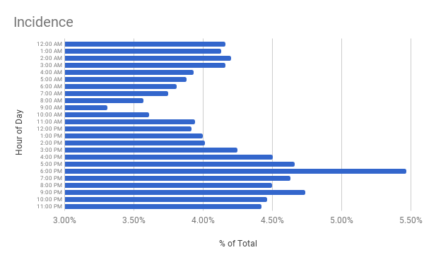
Incidence Type and Relationship with Clicks: Hour of Day
Looks like people are less likely to click on ads in the morning.
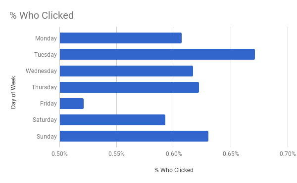
Incidence Type and Relationship with Clicks: Day of Week
Looks like on Friday people have better things to do than clicking on ads!
Addressing Imbalanced Classes on the Target Variable: Too Few Clicks
Our target variable (clicks) had imbalanced classes: only ~0.6% of all impressions were clicked on. We tried to address this issue by:
- Undersampling zeros: From ~69 million rows sample all impressions with clicks and only 2.5% of impressions without clicks:
- Final training dataset: ~2.1 million impressions, of which ~419K with clicks and ~1.7 Mil without (~1:4 ratio)
- Running predictions with and without class weights:
- rows with clicks get a weight of 0.8
- rows without clicks get a weight of 0.2
Predicting Clicks using Logistic Regression
Predictors used & in what form:
- Ad Size (categorical)
- Ad Type (categorical)
- Device Type (categorical)
- Exchange (categorical)
- Gender (categorical)
- Venue Type (categorical)
- State (categorical)
- Hour of the day (categorical)
- Day of the week (categorical)
- Hour/day interaction (categorical)
- Url (categorical)
- Age group (categorical)
- 15 dummy variables for top IAB categories (numeric)
Pipeline in Spark included the following:
- applying StringIndexer to every categorical (string) variable to label encode it;
- applying OneHoteEncoder to every label-encoded variable to create dummies for it.
15 IAB dummies were fed into the model as is.
All predictors were then standardized by default by LogisticRegression procedure (imported from pyspark.ml.classification)
Logistic Regression models tried & their diagnostics (for Test data): Ridge w/o regularization predicted best
The table below shows the diagnostics for several models we've run. Each of them took a long time to run and our attempts at running parameter grid search using cross-validation failed because the Amazon cluster we used was not large enough.
Area uROC stands for "area under Receiver Operating Characteristic Curve"
Area uPR stands for "area under Precision/Recall Curve"
We tried to run the models with and without case weights. We discovered that using class weights* is analogous to using no weights and then predicting clicks/non-clicks using a probability threshold that maximizes F1 measure: It raises Recall but reduces Precision & Accuracy.
Logistic Regression takeaways:
- Non-regularized Logistic Regression performed best - probably thanks to the large sample size
- The overall predictive power of our models could clearly be improved
- Additional feature engineering seemed warranted:
- Inclusion of categories with lower incidence
- Building additional columns for interaction between variables
- Inclusion of additional predictors, especially those related to user characteristics might help
Predicting Clicks using Random Forest
Predictors used & in what form:
- Ad Size (categorical)
- Ad Type (categorical)
- Device Type (categorical)
- Exchange (categorical)
- Gender (categorical)
- Venue Type (categorical)
- State (categorical)
- Hour of the day (categorical)
- Day of the week (categorical)
- Hour/day interaction (categorical)
- Url (categorical)
- Age (numeric - where missing value were coded as -999)
- Target group (categorical)
- 15 dummy variables for top IAB categories (numeric)
- Latitude & Longitude (numeric)
All categorical variables were label encoded using Spark’s StringIndexer. The encoded categoricals were then fed to the random forest classifier along with the unaltered numeric variables.
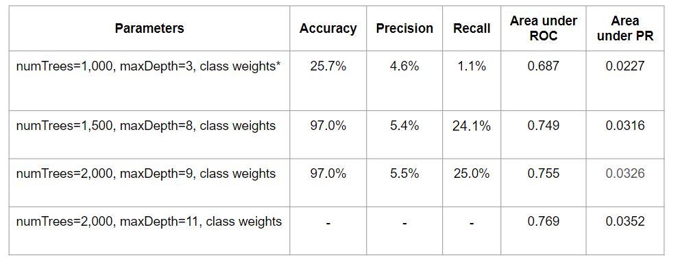
Random forest models tried & their diagnostics:
We did not have much time and each model took a long time to run. This is why we only ran a few Random Forest models. For the last model in the table below our several attempts to produce an accuracy table timed out, so that we are not reporting Accuracy, Precision, and Recall for it.
Random Forest takeaways:
- The overall predictive power of our Random Forest model was still not as high as desired
- Random Forest models took much longer to run, but performed somewhat better than Logistic Regression models - probably due to:
- high sparseness of our hotdeck-encoded predictors which might have impacted negatively the quality of Logistic Regression
- Absence of Latitude and Longitude as predictors for Logistic Regression
- The table below shows the results of the best Logistic Regression and Random Forest models:
Predictor Importance in Predicting Clicks
Logistic Regression (Ridge): Users’ “Target group” was the most important predictor of clicks
- User characteristics were the most important predictors of clicks;
- Users were more likely to click on videos;
- Users on PCs and Tablets were less likely to click on ads;
- Style & Fashion ads were clicked on more often and Health & Fitness ads - less often.
Top Positive Regression Coefficients for Logistic Regression:
- Top 30 positive coefficients: Target Group dummies
- Coefficient 31: State of Virginia dummy
- Coefficients 32-43: Target Group dummies
- Coefficient 44: ad type “3rd party video” dummy
- IAB18 (Style & Fashion) has the highest positive coefficient among IAB categories tested
Top Negative Regression Coefficients for Logistic Regression:
- Top 8 negative coefficients: Target Group dummies
- Coefficient 9: device type “Personal Computer” dummy
- Coefficients 10-36: Target Group dummies
- Coefficient 37: Washington DC dummy
- Coefficients 38-41: Target Group dummies
- Coefficient 42: device type “Mobile/Tablet” dummy
- IAB7 (Health & Fitness) has the highest negative coefficient among IAB categories tested
Predictor Importance: Random Forest
Predictor importance results from Random Forest were partially in line with logistic regression’s findings: Target group (with 1200+ levels) was the most important predictor.
The top predictors were:
Predictor & Importance Score (the importance scores for all predictors sum up to 100)
- Target group, .367
- Ad size, .121
- Landing page url, .104
- Exchange, .070
- Ad type, .057
- Carrier, .041
- IAB24 - “Uncategorized”, .035
- Hour of day, .026
- Age, .024
- IAB14 - “Society”, .023
Future Research Directions
- Consider creating dummies for more IAB categories and carriers, not just the highest incidence ones.
- Consider including additional device characteristics (e.g., we have not used device make & model).
- Consider building geographical clusters based on latitude/longitude - esp. when the right algorithms are implemented in Spark.
- Consider importing additional information - from BidRequests - as additional predictors of clicks.
- Consider using a larger cluster: our cluster was shared by 15 people and was too small for:
- merging all bidrequests with impressions and clicks, and
- running Cross-Validation


