Unsupervised dimension reduction and clustering to process data for pooled regression models
Abstract:
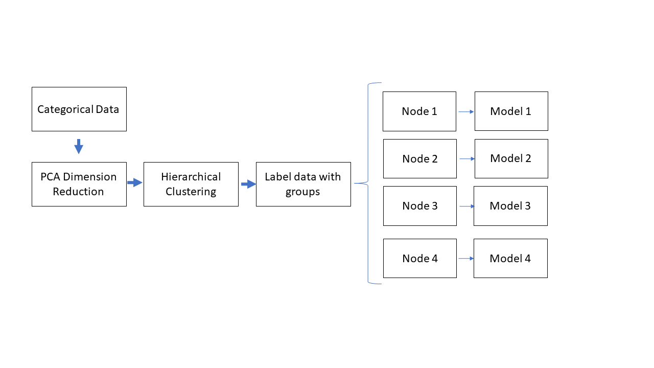
Unsupervised PCA and hierarchical clustering methods were used to group observations according to 41 dimensions of descriptive categorical features. Grouping the data into these 'nodes' resulted in an improved ability to describe the data with a simple multiple-linear model or identify outlier groups where alternative models are more suitable. A python class for thos method was also coded to enable grid-search-like parameter optimization in the future.
Results and Discussion:
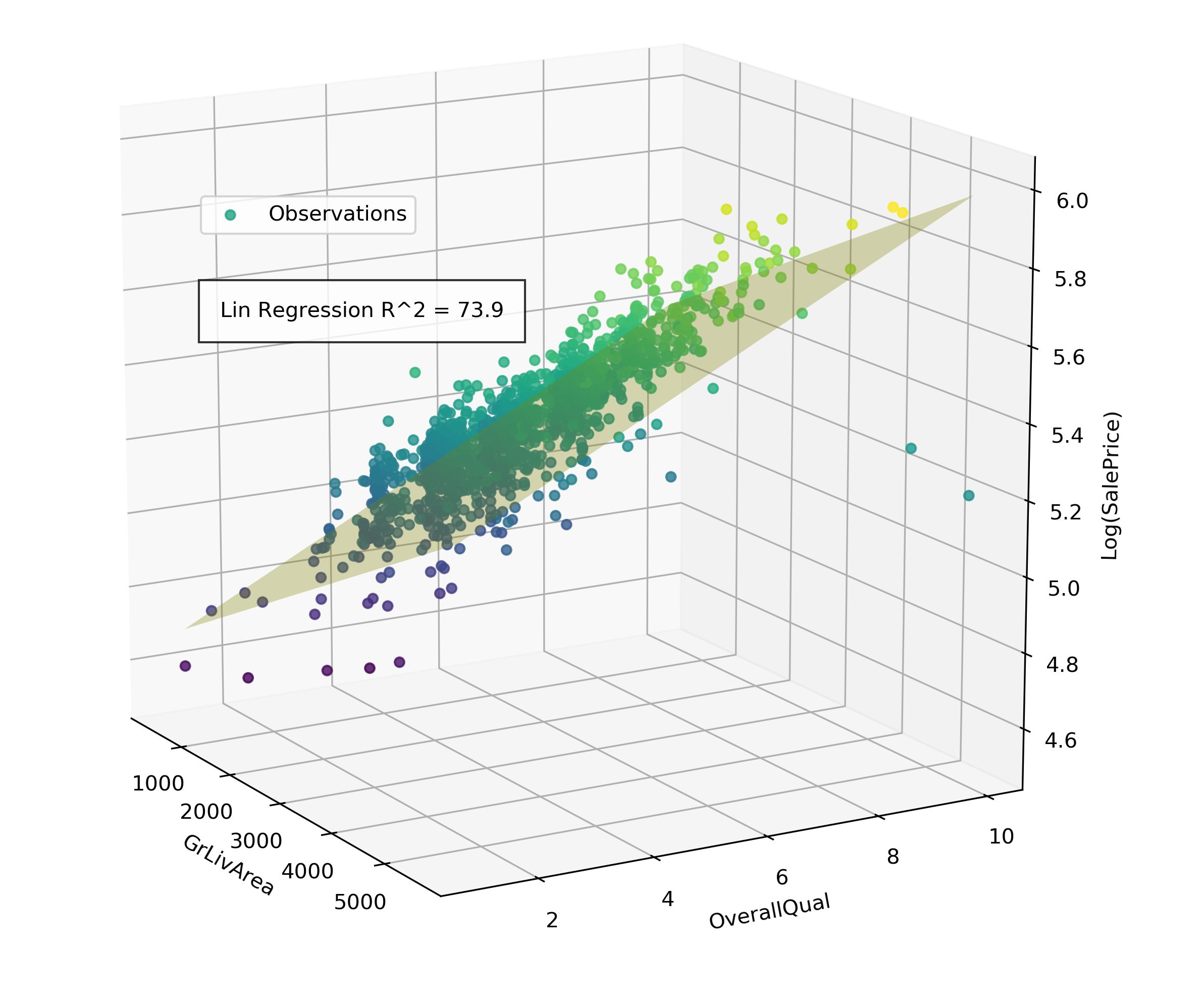
For this project, our team applied machine learning techniques on the Ames housing dataset in order to predict the sales prices of houses using 79 explanatory variables, defining 41 of these variables as categorical and 38 as continuous numerical. During initial EDA and feature selection process we aimed to better understand the data by fitting the data with only two continuous variables so that the data and model can be visualized in a 3D scatter plot. To select the two variables with the most predictive power for sales-price, a linear regression model was fit according to all possible two-variable permutations from the list of 38 continuous numerical features. When the whole training data set is considered, Ground Floor Living Area and Overall Quality Parameters were the best predictors for a house's sale price, but only explained 73.9% of the data variance. By using the 41 categorical features to identify groups within the dataset, we can subset the data into nodes with less variance and fit a model that better describes each particular subset of houses.

A simple linear regression model to display effect of house sales price as a function of great living area and overall quality. This simple model explains 74% of the housing price variation
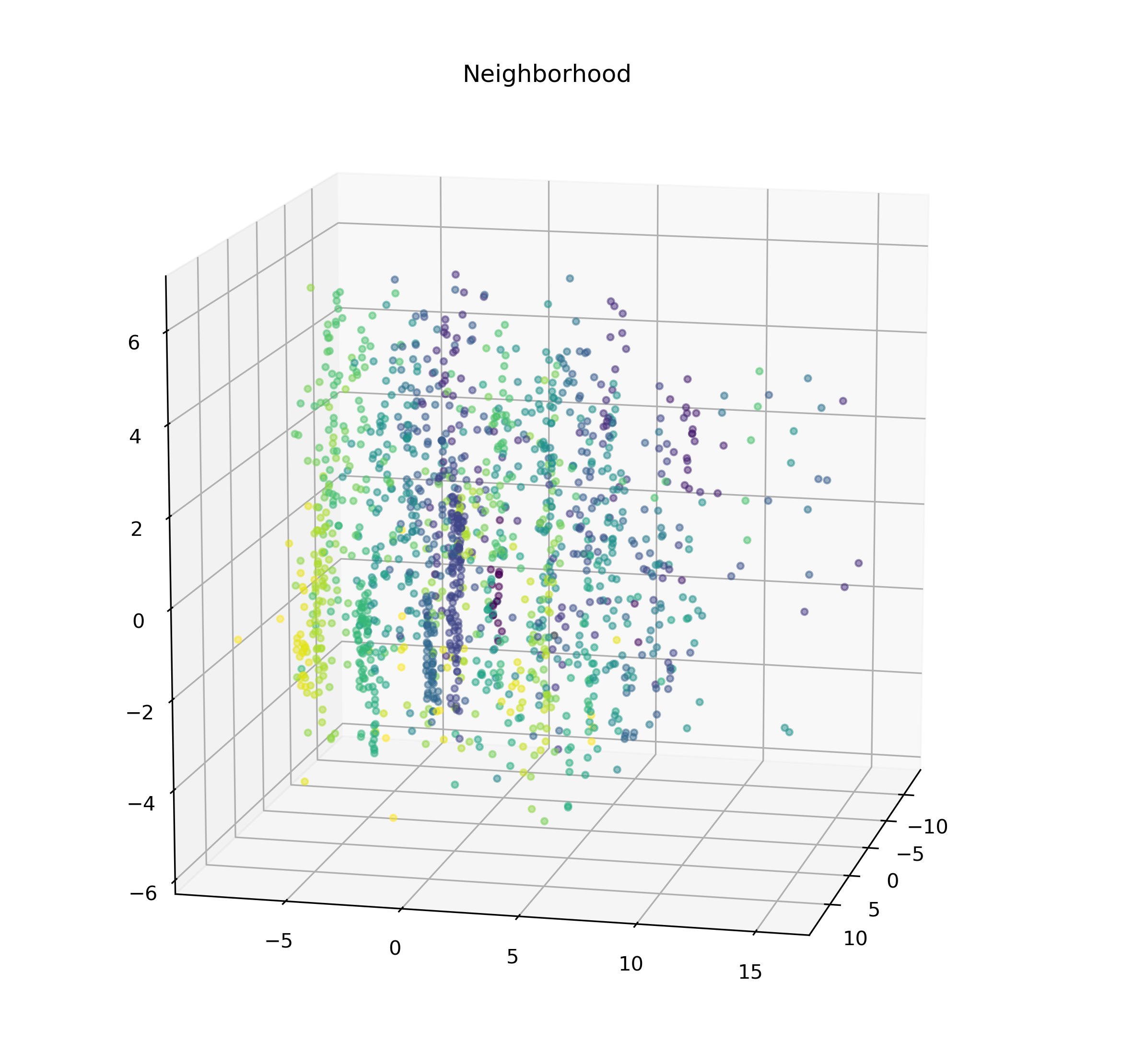
Since there are so many categorical variables and our domain knowledge of the Ames housing market is limited, we used unsupervised clustering methods to find patterns within the variables and group by those. PCA dimension reduction was first performed on the data set to avoid "curse of dimensionality" effects arising from a large number of categorical variables. PCA also has the added benefit of minimizing variables that do not contribute to the overall variance of the data, and by reducing the dimensions to 3, allows for a graphical representation of the clustering algorithms for intuitive modifications. A representation of the categorical variables condensed into 3 dimensions vis PCA can be viewed in figure 2 below:

Data arranged in 3 dimensional PCA space after being condensed from 41 dimensions of categorical features
Initial inspection of this graph indicates that majority of variation is represented by the new Y (vertical) dimension. In the X(width) and Z(depth) dimensions, the variations occur in defined clusters, resulting in the data forming vertically oriented striations. Due to the anisotropy of the clusters, a hierarchical clustering algorithm with a K-nearest neighbor connector parameter was used to define groups without breaking up the striations into parts. Python sklearn AgglomerativeClustering package was used to perform clustering. In the example reported here, the number of clusters was set to 6, using a Ward linkage criteria, and a connectivity array generated by the kneighbors_graph package where n_neighbors parameter is set to 20.

Coloring PCA condensed observations by neighboorhood gives some clues as to what factors influence dimension condensation and grouping
The clustering generated by the PCA / Clustering method performed fairly well in distinguising the vertical 'striations' in the grouping. To draw some parallels between the unsupervised clustering and what they mean in relation to the house characteristics they are based on, the clusters were also colored by each categorical variable. Several of these colored scatter-plots resembled the unsupervised groupings, suggesting those particular house characteristics play a larger role in determining the final PCA vectors for each data point. In particular, coloring by neighborhood highlights the vertical grouping visually similar to the unsupervised method, suggesting that the neighboorhood is an important factor by which to sub-set these houses. More numerically rigorous methods of determining overall "contribution" of each factor to the final PCA dimensions will need to be devised for this application.
These 6 groups were used to subset the continuous numerical data in order to determine which top two factors are the best predictors for the sale-price ing each group, assuming a simple 2-factor linear regression model
| Group | Top 2 predictors for SalePrice | Lin Regression Score |
| 1 | Overall Quality : GrLivArea | 79.5 % |
| 2 | Overall Quality : GarageArea | 68.2 % |
| 3 | Overall Quality : GarageCars | 73.5 % |
| 4 | Overall Quality : 1stFlrSF | 62.5% |
| 5 | Overall Quality : GarageCars | 85.9 % |
While some nodes exhibit a better fitting with linear regression than others, there is no cumulative difference in accuracy of fitting models to these groups versus treating the data as a whole. However, this is an initial iteration of this proof of concept and crucial parameters such as n_nodes, PCA dimensions, and KNN connectivity parameters have not been optimized. Putting these methods were coded into a python class which can assist in applying a grid-search-like optimization process to determine the best clustering parameters to maximize the accuracy of simple linear regression models. Please refer to the "MC_regressor_Code.ipynb" under the following GitHub link: https://github.com/dgoldman916/housing-ml.
Next steps:
At this point, the ability to train and classify new data into the model is the key functionality lacking from this 'proof-of-concept'. When introducing a test set of data, the new data must now be classified into labeled groups, according to a trained set of parameters. This will require a supervised clustering method, likely in the form of a decision tree or SVM. After this function is added, it can be applied to the rest of the group's work-flow. The intended final iteration would be used to fit more complicated models across the nodes and pool the results of these models together.


