Kaggle Competition : Predicting House Prices in Ames, Iowa
In recent years, machine learning has been successfully deployed across many fields and for a wide range of purposes. One of its applications is in the prediction of house prices, which is the putative goal of this project, using data from a Kaggle competition. The dataset, which consists of 2,919 homes (1,460 in the training set) in Ames, Iowa evaluated across 80 features, provided excellent learning material on which to perform exploratory data analysis, imputation, feature engineering, and machine learning (linear-based models, tree-based models, and ensembling). Our main objectives for the project were 1) to gain facility in the end-to-end process of a data science project in a collaborative environment and 2) to better understand the implementation and evaluation of various supervised machine learning techniques.
Workflow
Our workflow consisted of a full development cycle divided into five stages: exploratory data analysis and pre-processing, feature engineering, modeling, hyperparameter tuning, and ensembling. The following is a workflow chart illustrating the five stages:
The machine learning models we used for this project were the following:
- Linear-Based Models
- Simple Multi-Linear
- Ridge Regression
- Lasso Regression
- Tree-Based Models
- Decision Trees
- Random Forests
- Gradient Boosting
- Ensemble Models
- Ridge Regression + Lasso Regression + Random Forests
Exploratory Data Analysis (EDA)
To gain a sense of the relationship of the features with each other and with house sale prices, the target variable, we employed a diverse set of data visualization tools, including the following: density plots, scatterplots, boxplots, and correlation plots.
The first EDA we performed was to examine the distribution of the home sale prices. The histogram of home sale prices appeared to be right-skewed. We therefore performed a log transformation of the home sales prices to make the distribution more Gaussian. The following are histograms of home sales prices before and after the log-transformation: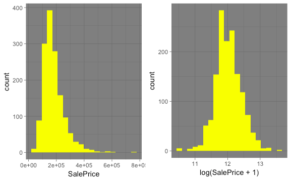
The second EDA we performed was to create a matrix of Table Plots of the features (x-axis) against the target variable (home sales price). To interpret these density plots, in general we looked for two things: 1) a linear relationship between the feature and the target variable and 2) variation in the density of each feature value versus home sales price. The following is an example of some of the density plots for features we found to have a strong relationship with home sale price:
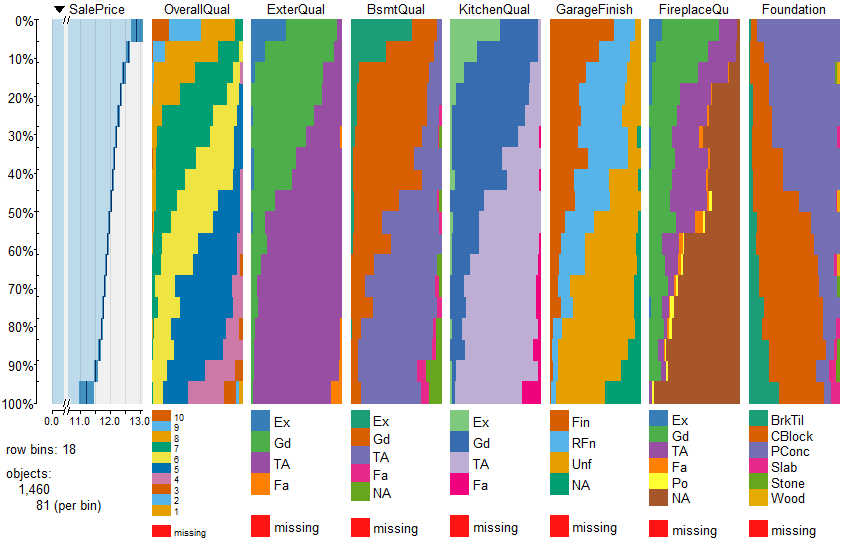
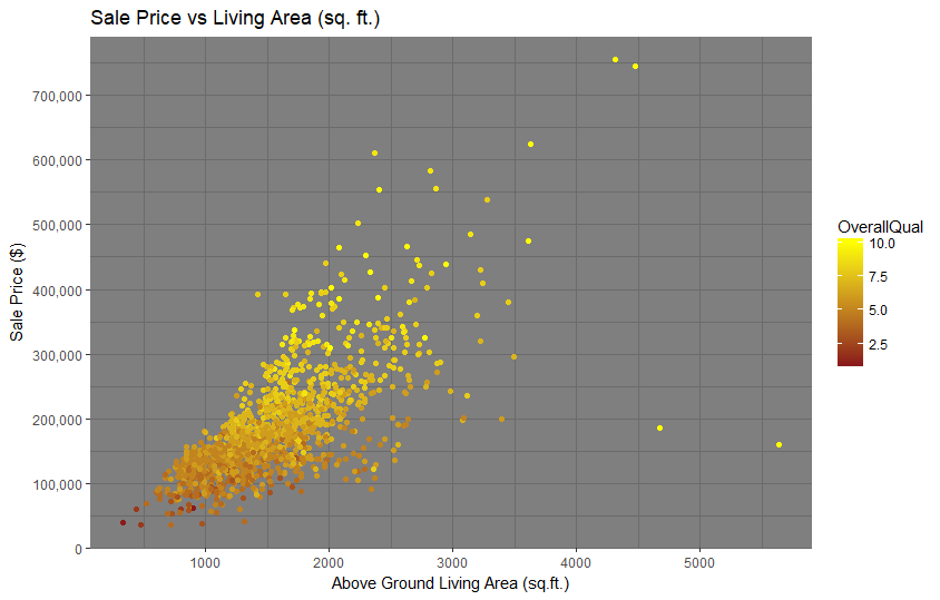
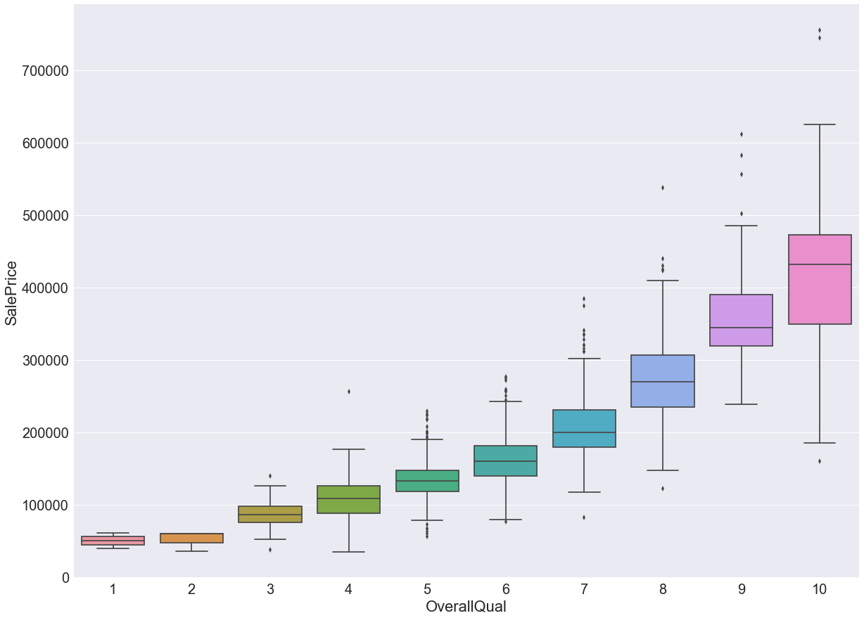
 Other plots we used to explore the relationship between features and home sales prices included scatterplots and boxplots. Examples include the following:
Lastly, we also explored the correlation between the various features using correlation matrices. The following correlation matrix shows the correlations between some of these features, with darker colors indicating higher correlations.
Based primarily on these various EDA results, we narrowed the list of features to around twenty which we considered in our base multiple linear regression model. This will be discussed later in the blog post.
Data Cleaning
In order for machine learning algorithms to provide meaningful insights, we needed to ensure that the data was relatively clean. For our dataset, we had to change some feature types and also handle missing values.
Type Conversion
First, we had to change the data types of the below features from numeric to string.
| Features |
MSSubClass, OverallCond, OverallQual, GarageCars, YrSold, MoSold |
The values for each feature above represent different categories and not different amounts of something. This is easiest to see in the case of MSSubClass, where the numbers encode different categories of houses, such as 2-Story 1946 and Newer (60) and 2-Story 1945 and Older (70). It is harder to discern in a feature like GarageCars, where each value seems to count something (cars) but in actuality represents the garage capacity, and therefore represents a category.
Missing Values
We used the below strategies for dealing with missing values.
Flagging as 'None'
| Features | Alley, BsmtCond, BsmtQual, BsmtExposure, BsmtFinType1, BsmtFinType2, Fence, Functional, FireplaceQu, GarageCond, GarageFinish, GarageQual, GarageType, MasVnrType, MiscFeature, MSSubClass, PoolQC |
In many cases, we want the model to treat observations with missing values as a separate category. For example, we know from the data description that a missing value for ‘PoolQC’ means that the house does not have a pool. It is important to let the algorithm know that some houses do not have pools, because this may affect their value, so we flag the missing values as ‘none’. The only exception is 'Functional': we still want to flag the missing values for this feature, but we assign the value ‘typ’ instead of 'none' because the data description says that missing values here mean ‘typical functionality’.
Impute Zero
| Features | BsmtFinSF1, BsmtFinSF2, BsmtUnfSF, BsmtFullBath, BsmtHalfBath, GarageArea, GarageCars, TotalBsmtSF |
For numeric features, when the house does not have attribute being measured it usually works to impute zero. It makes sense, for example, that the area of a missing garage is zero square feet, and that a missing basement has zero bathrooms.
Impute the Mode
| Features | Exterior1st, Exterior2nd, KitchenQual, Electrical, MSZoning |
For these categorical features, we knew the house had the attribute being measured, so we could not impute 'none'. In all the cases, there was one dominant value for most of the data and so we decided to impute the mode as the value of the missing data because, assuming the data are missing completely at random, it is probable that they (like most of the observations) have the most typical value.
Impute the Median by Neighborhood
| Features | LotFrontage |
For LotFrontage, we needed to impute a value because it does not make sense that a house is actually missing the attribute. Instead of imputing the median value for the entire dataset, we decided to impute the median for the neighborhood the house is located in to give us a more accurate estimate.
Features Engineering
It is usually the case that quality features produce better models, and one way to improve the quality and variety of features is to strategically create new ones by combining existing ones. However, just adding more features isn’t necessarily helpful because one might encounter such issues as multicollinearity, the ‘curse of dimensionality’, increased processing time, and overfitting. Since there is a cost to adding features, we had to exercise judgment in which ones to add.
Derived Features
| Features | TotalSF = TotalBsmtSF + GrLivArea |
| HighQualFinishedSF = TotalSF - LowQualFinSF | |
| TotalBaths = FullBath + BsmtFullBath + .5(HalfBath + BsmtHalfBath) |
Derived features are obtained by performing arithmetic on two or more similar features to produce another one. For example, we added several similar features describing the number of baths to obtain the overall number for the house, and we obtained total square footage and total high-quality square footage by performing arithmetic on features that measured square footage.
Feature Interactions
| Features | OverallQuality*OverallCond | ExteriorQual*ExteriorCond |
| BsmtQual*BsmtCond | GarageQual*GarageCond | |
| HeatingQual*HeatingCond | SaleType*SaleCond | |
| Neighborhood*BldgType |
There are sometimes features in the dataset that interact with each other, which happens when a change in one feature increases or diminishes the effect of another feature. For example, if you have two houses with a '5' for 'ExternalCondition' but different scores (a '2' and a '10') for external quality, the '5' should be weighted differently based on the quality score. The same condition score means something different when a house is low quality versus high quality, and the same applies vice versa (the same quality means something different when it is of low condition versus high condition). The top three rows in the table above list features that, like 'ExteriorQual*ExteriorCond', capture interactions between two different measures of the same thing.
We included the feature in the last row because we think there may also be an interaction between the type of house and the neighborhood. Maybe townhouses are predictably cheap in one neighborhood but predictably expensive in another. And, conversely, maybe a particular neighborhood tends to have expensive townhouses but cheap single-family houses.
Multiple Linear Regression
For our base model, we used a multiple linear regression model. We selected 20 features that we believed were the most promising based on the EDA we performed as described previously. We further narrowed the list of 20 features by organizing them into five main categories based on our understanding of how a typical home buyer or investor would assess a home. The table below summarizes our analysis:
| Location | Style | Condition | Size | Other |
| Neighborhood | HouseStyle | OverallQual | GrLivArea | SaleCondition |
| MSZoning | Foundation | OverallCond | 1stFlrSF, 2ndFlrSF | SaleType |
| GarageFinish | YrBuilt | FullBath | ||
| Paved Drive | ExterQual | TotRms | ||
| BsmtQual | GarageCars | |||
| GarageArea |
The features highlighted in red were the ones we ultimately selected to run in our initial multiple linear regression model. With the exception of 'GrLivArea', all the features are categorical features. Before dummifying these categorical features, we further grouped the values of these categorical features into quantiles based on the relationship of each feature with the target variable. One reason is to limit the number of explanatory variables in our model after dummification so as to lower the possibility of multicollinearity issues. We also performed a variance inflation factor (“VIF”) analysis to gain further comfort. In general, a VIF score above 5 indicates that multi-collinearity might be an issue. After dummification, all the explanatory variables we chose had a VIF score below 5.
Our model selection process was the following:
- We split the training set 80%/20% into sub-training and test sets, respectively.
- We fit the model against the 80% sub-training set and then tested this against the remaining 20%.
- After testing, we then fit the model to the entire training set.
The R-squared values across the various models we trained and tested ranged from approximately 80 percent to 81 percent. As part of our residuals analysis after we fit the model against the entire training set, we examined if there were any influential points that may have had an outsized influence on the regression. As the following graph shows, there are two observations (#523 and #1298) which stand out based on their influence as represented graphically by the sizes of their circles.
Based on further review, we noted that the sale prices for these two houses were very low relative to their living areas, even in comparison with other houses in the Edwards neighborhood, where they are located. Because we couldn’t detect any patterns or features that might explain this, we made the decision to exclude these two data points from our analysis. After re-running the regression without these two data points, we arrived at a R-squared value of around 81 percent for the entire training set. We further note that the regression is significant at the 5 percent significance level and that the features with the highest absolute beta coefficient values were the top quantiles in terms of house quality and type of sale (for example, normal sale or a short sale).
Ridge and Lasso Linear Regressions
The process we used to train and test the Ridge and Lasso linear regression models was similar to the one we used for the multiple linear regression model. The major difference was the further complication of tuning the model hyperparameter that affects the L1 and L2 penalty terms. The following was the process we used:
- We split the training set 80%/20% into sub-training and test sets, respectively.
- We used a grid search in combination with a 5-fold cross-validation process to select our hyperparameter.
- We fit the model against the 80% sub-training set and then tested this against the remaining 20%.
- After testing, we then fit the model to the entire training set.
Ridge Linear Regression:
For the Ridge linear regression model, we expanded our features list to include many of the interactions described previously. Given the presence of the L2 regularization term, we felt reasonably comfortable with expanding our features list. The following graph illustrates the result of our grid-search analysis used to tune the hyperparameter. We note that the optimal hyperparameter, in which the root mean squared error is at the minimum, is an alpha of 18.7.
Using an alpha of 18.7, we note that the R-squared values across the various models we trained and tested ranged from approximately 91 percent to 94 percent. We also note that the R-squared value is lower for the test set than the R-squared value for the training set, which indicates that there may be some overfitting. Consistent with the results from the baseline multiple linear regression model, the features with the highest absolute beta coefficient values were those related to the quality and condition of the homes, the neighborhood, and the interaction between them.
Lasso Linear Regression:
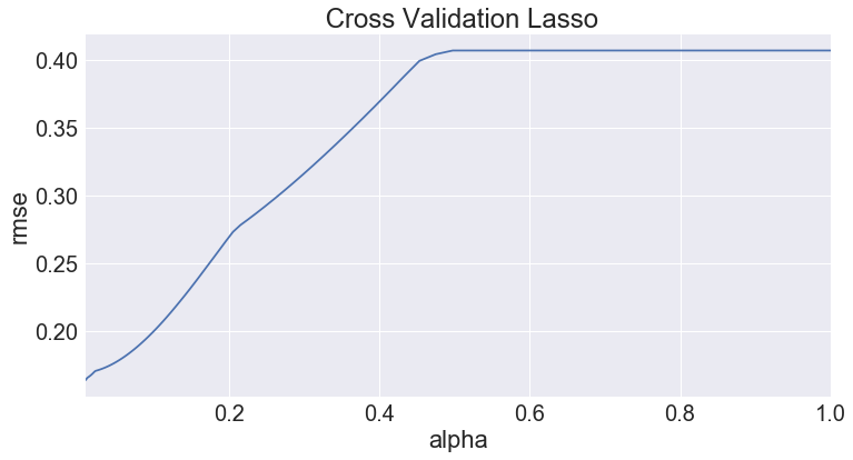
For the Lasso linear regression model, we regressed the same set of initial features from the Ridge model against house sales prices. We also employed the same hyperparameter tuning process but interestingly, the optimal hyperparameter for the L1 regularization term was much smaller at 0.01. The following line chart provides a graphical representation of our grid search results.
Using an alpha of 0.01, we note that the Lasso performed worse than the Ridge model in terms of predictive accuracy. The R-squared value for the Lasso models we trained and tested hovered around 84 percent. However, consistent with the results from the previous linear regression models, the features with the highest absolute beta coefficient values were those related to the quality and condition of the homes and neighborhood. It is also interesting to note that the combination of home sale type and sale condition had the highest absolute beta coefficient value.
Tree-Based Models
Tree-based methods empower predictive models with high accuracy, stability and ease of interpretation. Unlike linear models, they map non-linear relationships quite well. They are adaptable to solving either classification or regression problems.
We developed three classes of tree-based models: decision trees, random forests and gradient boosting. It was highly interesting to evaluate and compare the distinctive characteristics and performance of each of the three separate tree-based models.
To better understand the underlying behaviors, we plotted the root mean-squared log error ("RMSLE") against a range of hyperparameter values. These plots were instrumental in:
- Visualizing the underlying trends as hyperparameters are varied
- Identifying the regions of Bias vs Variance trade-offs
- Acquiring an estimated range of values to feed into the cross validation grid search algorithm
Subsequently, cross validation grid search was performed on each tree-based model with their respective hyperparameters. This resulted in the selection of the optimal hyperparameters based upon the average RMSLE score against the test set.
It was interesting to note the distinction between each of the tree-based models by examining their prediction profiles. Evidently, decision trees exhibit clear discrete steps in the prediction plots owing to its simplistic model. The random forests and gradient boosting models achieved a better fit to the actual prediction profile from the training set. This is attributable to the bagging and boosting procedures in the random forests and gradient boosting models, respectively.
 Furthermore, the variable importance plots gave valuable insights on the various tree-based models. It uncovers which variables were ultimately utilized by the models and their relative importance. Here are some interesting takeaways:
- Decision trees and random forests converged on the same number of important variables.
- Random forests resulted in a different order of variable importance. This is attributable to its random feature selection at each split in the tree.
- Gradient boosting incorporated the most number of important variables. The boosting process enables “weaker” features to be included alongside the “stronger” features.
Ultimately, gradient boosting combines weak learners to form a more accurate and robust decision ruleset.
Ensemble Model
After creating the linear and tree-based models above, we decided to combine them in an ensemble in order to increase the prediction accuracy and improve the overall confidence level of the predictions. The various models capture different aspects of the dataset, such as outliers, thereby making the ensemble more robust.
A number of transformations and imputations were made to the dataset in this stage in addition to those made in the earlier stages before running the models in the ensemble. These included un-skewing all features with a skewness greater than 0.75 and removing outliers. These outliers were detected visually from the plots and confirmed using the Bonferroni outlier test.
We used the StackingRegressor from the mlxtend package. The ensemble model consisted of lasso regression, ridge regression, and random forests models and used lasso regression as the second level model (meta-regressor). This is illustrated in the image below.
Results
The following is a summary of the RMSLEs for the various models against the public test set and also against Kaggle's private test set used to score the submissions.
| RMSLE | |||
| Models | Test | Kaggle | |
| Linear Based | Multi-Linear | 0.1641 | 0.1788 |
| Ridge Regression | 0.1110 | 0.1290 | |
| Lasso Regression | 0.1370 | 0.1414 | |
| Tree-Based | Decision Trees | 0.1910 | 0.1882 |
| Random Forests | 0.1358 | 0.1465 | |
| Gradient Boosting | 0.1184 | 0.1245 | |
| Ensemble | Ridge, Lasso, RF | 0.0949 | 0.1251 |
Conclusion
Based on our experience with this project, we were able to gain valuable insights on the application of a range of machine learning models. For example, we discovered that features engineering and hyperparameter tuning proved to be vital steps and could have a big impact on the performance of the machine learning models. Also ridge regression and lasso regression within generally outperformed the tree-based models, with the exception of gradient boosting. This is most likely due to the size and nature of the dataset, which appears to lend itself more to the application of regression models.


