Data Analyzing Iowa Housing Prices Using Machine Learning
Project GitHub | LinkedIn: Niki Moritz Hao-Wei Matthew Oren
The skills we demoed here can be learned through taking Data Science with Machine Learning bootcamp with NYC Data Science Academy.
This study was completed as a project for the NYC Data Science Academy in which each group entered the same Kaggle Competition. This study was conducted by three data science fellows: Benjamin Rosen, Oluwole Alowolodu, and David Levy.
Housing Dataset
The dataset obtained from Kaggle consisted of housing data for the city of Ames, Iowa which had 1460 observations with 80 variables. The purpose of the study was to predict the sale prices of houses. From the start, it was clear to our group that the main challenge to this study would be dealing with the high number of features, with the majority of them being categorical. Before the features were analyzed, however, attention was first directed towards the missing values in the dataset.
Missingness Imputation

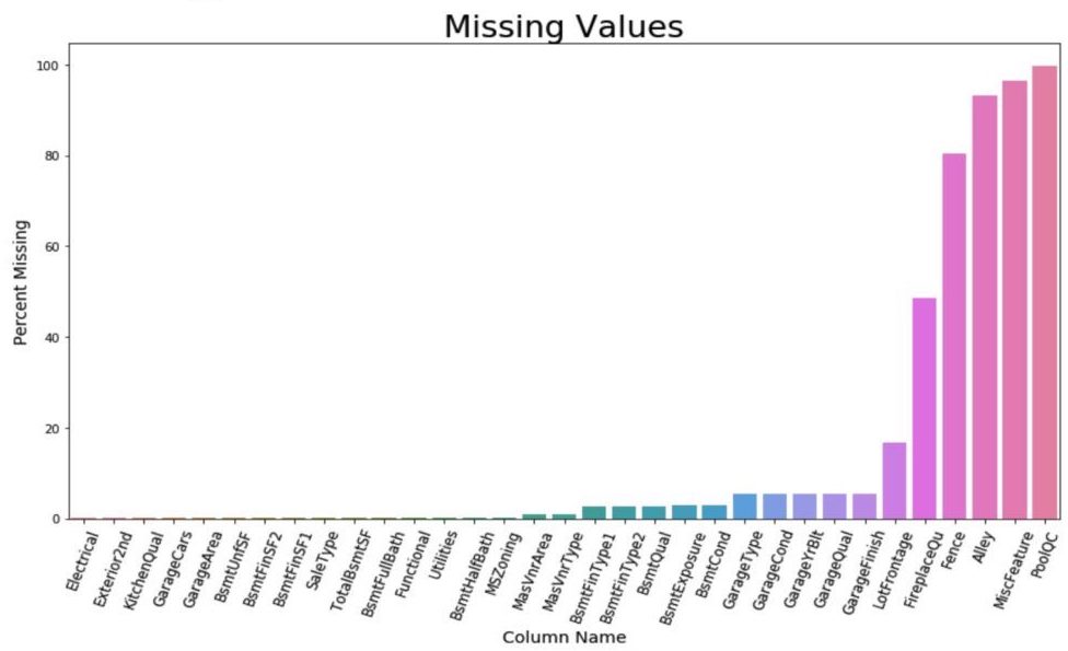
After combining the train and test set (given separately from Kaggle), 34 columns had missing values. In order to impute missing values, we used a few different methods based on an understanding of the data, the category type and the number of missing values. Categorical variables that accounted for house features, such as alley, fence, and garage quality, commonly had missing values, which indicated the house did not have a particular feature. Thus, the missing value was not an unknown value, but an additional category which could be coded as "No Feature."
For example, in the alley column, the column value was "NA" if a house did not have an alley next to it, as opposed to its usual meaning that it was an unknown value. Numerical features, such as lot frontage, basement square footage, and masonry veneer area, typically only had a few values missing (usually at random), and so a median value was imputed for these columns.
For lot frontage, a numerical column used to account for the linear feet of street connected to the property had many missing values so we imputed the most common value found in that specific neighborhood for the missing value. The researchers determined that this imputation method would create the most accurate representation for the lot frontage distribution in Ames, Iowa.
Removing Outliers


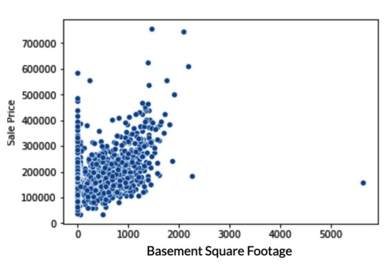
Outliers are considered to be values that deviate from the mean so substantially that it leads to inaccurate models when used to predict the dependent variable, which is the sale price of a house. In the above graphs, outliers can be shown by identifying the select points in the graph that clearly do not follow the general trend of the graph. Houses with either a basement square footage greater than 5,000 square feet, above ground living area greater than 4,700, and lot frontage greater than 300 feet were removed from only the training dataset, which resulted in a removal of three houses.
Feature Engineering
Creating New Variables
One of the most challenging aspects of this project was dealing with the high number of dimensions, with many of those being categorical. The first task that was focused upon was creating new variables from the existing ones. The dataset included three different columns which were represented by year: year built, garage year built, and remodeling year.
Because the majority of observations had equal values for all three, binary variables were created to capture differences in years, which would indicate that there was some kind of renovation done which could undoubtedly influence the subsequent sale price. Variables were also created to capture the differences between the years to in hope that it would be statistically significant.
Additionally, binary variables were created for houses built before 1960 and after 1980 to determine if houses classified as "old" and "new", respectively, had significant influence, on the price. The remaining columns were created to capture whether houses merely having a certain feature (binary), regardless of magnitude, influenced its price.

Normalizing Skewed Distributions
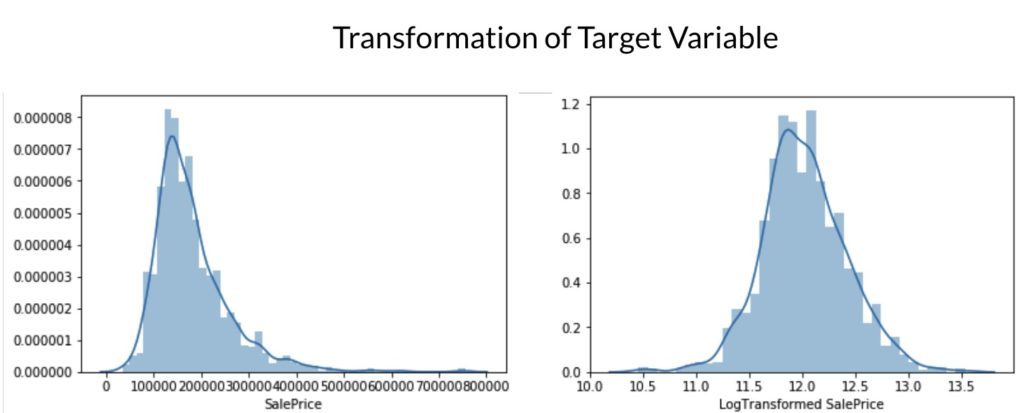
Normal distributions are assumed for linear regression, therefore, it was necessary to ensure that this was the case for all variables. Variables that were right-skewed or left-skewed were normalized using the log transformation or the Box-Cox transformation. As can see below, log transformation normalized the distributions of Lot Area and Above Ground Living Area.

Similarly, the dependent variable, Sale Price, was log transformed due to its right-skewed distribution.

Lastly, the only column dropped from the dataset was the year that the garage was built. As explained earlier, the values were highly correlated with the year the house was built, and we accounted for the difference between the two columns by creating additional binary and numeric variables.
Fitting Models To The Data
Seven different models were used to determine the best method for prediction, however, only the best three will be explored extensively. We primarily used Scikit-Learn's Grid Search CV to find the optimal parameters for each model.
Ridge Regression
Before running a grid search for the ridge regression, the number of folds for cross-validation was explored. The industry standard tended to be either 5 or 10, with the majority using the latter, however, we still explored this task graphically.

As the number of folds increases, the mean error remains relatively constant, while the standard deviation steadily increased. While trying to minimize error and variance, a value of 10 folds was chosen, which is in accordance with our prior knowledge.
As expected, as the alpha hyperparameter increases, coefficient converges (but do not equal) zero due to the fact that alpha controls the magnitude of penalization.

After grid searching for optimal parameters, alpha was selected to be 10, which allows the coefficients to be shrunk enough in order to avoid over-fitting the training data. The ridge regression had an R Squared of 0.9418 and a root MSE (Mean Squared Error) of 0.1133, determined by cross-validation and 0.11876, determined by Kaggle.
ElasticNet
The next model evaluated was Scikit-Learn's ElasticNet algorithm. The most influential hyperparameters of the ElasticNet are alpha, which is essentially the weight for penalization, and the L1 ratio, which can incorporate both the L1 and L2 penalties depending on its value. The grid search resulted in a value of 0.1 for alpha and .001 for the L1 ratio. As displayed by the graph below, as the L1 ratio is increased, coefficients converge at a higher rate than in the ridge regression, most likely due to L1 ratio's nature of incorporating both the Lasso and Ridge penalty parameters.

The R Squared of the ElasticNet was found to be 0.9209, while the cross-validated root MSE was 0.11204 and Kaggle's value was .12286.
Support Vector Regressor
Finally, a support vector regressor was used to predict the housing prices. The three parameters of focus were gamma, C, and epsilon, which all are related to the level of coefficient penalization. We expected the grid search to find a low value for gamma because this would avoid overfitting the training data. It found an optimal parameter for gamma to equal 10-6, which is much less than the default value of .0015 (1 divided by the number of features).
C was found to be 1000 which is not necessarily restrictive of parameters, but it establishes a "hard margin", meaning that the interval between the value and it's prediction instills a strict penalty, as opposed to a flexible one. Finally, epsilon was found to be zero which put a penalty on all error terms. The graph below confirms the grid search's finding of a low value for gamma, and a high value for C in which both result in a low root MSE.

Feature Importance Obtained From Tree-Based Models
Gradient Boosting Regressor and Random Forest models were both run using SciKit-Learn's framework. There are many commonalities between the two rankings with Overall Quality, Above Ground Living Area, and Total Basement Square Footage in the top three for both models.

Unexpected Results
The 15 variables selected as important did not entirely match our initial hypotheses. Lot Area was expected to be ranked of greater importance and we were surprised to see it outside of the top ten. Additionally, based on observations made from an initial correlation matrix, the following variables were expected to be important but failed to acheive a high ranking: neighboorhood, proximity to the closest railroad, and building type (which specifies the number of families).
Opportunities For Future Research
One source of potential bias was identified in the feature importance graphs. The values for the number of garage cars and garage area were included in the final models, which may have biased the models due to their collinear nature. The penalized linear regression models, such as the ElasticNet, Lasso, and Ridge, account for multicollinearity between features, but the tree-based models failed to do so.
Removing one of these variables may lead to a more accurate model with less bias. This can be done by using Principal Component Analysis (PCA) or inspecting the Variance Inflation Factors (VIF) in order to produce a model with uncorrelated independent variables. Finally, the model performances were assessed using R Squared and Root MSE. Other valid evaluation metrics that could be used in the future are the AIC (Akaike information criterion) and BIC (Bayesian information criterion).
Final Model Comparison
The following chart displays the final evaluation of the study's models, assessed by explained variance and root MSE, and their optimal parameters. The team's ridge model ranked 847 of out 4,086 submissions which placed this study in the top 21% of all submissions.

Code for this project can be found here.
Kaggle Competition: Kaggle Link

