Higgs Boson Kaggle Machine Learning Competition
Contributed by Wanda Wang, Rob Castellano, and Ho Fai Wong. They are currently in the NYC Data Science Academy 12 week full-time Data Science Bootcamp program taking place between April 11th to July 1st, 2016. This post is based on their fourth class project - Machine Learning (due on the 8th week of the program).
I. Introduction
The ATLAS experiment and the CMS experiment recently claimed the discovery of the Higgs boson, a particle theorized almost 50 years ago to have the role of giving mass to other elementary particles. The ATLAS experiment at the Large Hadron Collider (LHC) at CERN provided simulated data used by physicists in a search for the Higgs boson for the Higgs Boson Machine Learning Challenge organized on Kaggle.
The immediate goal of the Kaggle competition was to explore the potential of advanced classification methods to improve the statistical significance of the experiment. Specifically, the Higgs boson has many different processes through which it can decay. When it decays, it produces other particles via specific channels. The challenge consisted in developing a model to classify events corresponding to a Higgs to tau tau decay channel (signal) versus other particles and processes (background).
The Higgs Boson kaggle dataset was used in this analysis. The data exploration and machine learning was performed in R. All the code is available here.
II. Exploratory Data Analysis
Missingness
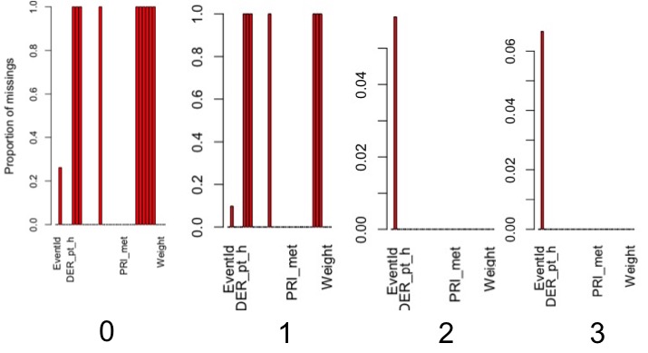
We carried out exploratory data analysis and quickly noticed that 11 of the 30 features contained missing data (initially recorded as -999). Upon closer inspection, 10 of the 11 features were related to jets (pseudo-particles) and specifically to the number of jets for a given event (recorded in the PRI_jet_num factor variable):
- 0 jets: features related to jets were all missing data, understandably
- 1 jet: features related to primary jets were no longer missing data, but those related to 2 or more jets were still missing
- 2 or more jets: all features related to jets contained data
In other words, the jet number can be treated as a factor for missingness in these 10 features. The 11th feature with missing data was DER_mass_MMC (unrelated to number of jets), and was due to the topology of the event being too far from the expected topology (not an error in measurement). The figure below shows the proportion of missingness as a function of jet number.
Given these observations on the missing data, we decided not to perform advanced imputation moving forward.
Principal Component Analysis
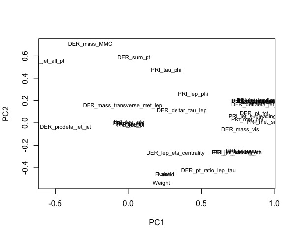
We then carried out Principal Component Analysis (PCA) to get a better understanding of the relationship between the 30 different features. When the features are plotted along the first principal component versus the second principal component (Figure below), it is clear that there are several clusters of features. These clusters of features indicates that collinearity is present among many of the features.
 One relationship that particularly stood out across 9 principal components was between the feature derived mass and label (whether the particle is signal or background noise) which showed that the derived mass and label have a very strong relationship.
Importance of Mass
Looking deeper into the mass features, mass seems a good predictor of presence of the Higgs Boson since the derived mass of the Higgs Boson is different from other (Z and W) Bosons and subatomic particles. Derived mass was the differentiating feature that the CERN scientists used to determine whether a particle was a Higgs Boson particle or not. The upper figure below is taken from the Science paper where the CERN scientists explain their findings. The small blue area centered at 125 GeV represents signal from Higgs Boson while the red area centered at 98 GeV represents background noise from Z Bosons. The lower figure below, we reproduce this graph using the simulated data set from the Kaggle competition. The simulated data set has a higher signal to background ratio than found experimentally to help with the model fitting. The dataset is weighted to take this discrepancy into account.
Correlation Matrix
Plotting a correlation matrix indicates strong covariance among subsets of the features. This was taken into consideration when we explored using predictive models in the next section.
Logistic Regression
We performed an initial logistic regression to further explore the dataset and investigate variable importance.
Initial Feature Engineering
14 Features with long-tailed distributions were log transformed to reduce the positive skew towards smaller values, generating a more uniform distribution e.g. DER_mass_jet_jet, the invariant mass of the two jets. This feature engineering to create more normal distributions can help with the model fitting. Although this feature engineering was not specifically used in our models, we would consider performing log transformations of these 14 features in the future.
Variable Importance
The bar charts below illustrate the variable importance obtained from logistic regression for the saturated (30 variables) and the stepwise BIC model (18 variables). To note, 12 DER prefixed variables were kept as a result of the stepwise model, compared to only 6 PRI variables which remained. Derived variables thus have more descriptive value.
Choice of AUC as model fit metric
In order to iteratively tune, improve, and combine various machine learning algorithms, a stable and reliable model fit metric was crucial. The Kaggle competition used approximate median discovery significance (AMS) scores to assess model performance but after performing online research and running a few simulations, it seemed that the AMS metric wasn't very stable. We opted instead to use the receiver operating characteristic area under the curve (AUC) which maximizes the true positive rate while also minimizes the false positive rate, and produces a stable, smooth and continuous function unlike AMS.
Logistic Regression Analysis
The logistic regression led to the following results:
- Saturated Model: R.Squared: 0.20227
- Stepwise BIC model: R.Squared: 0.20223
In comparing the deviance of the stepwise model to the deviance of the saturated model, the p-value for the overall test of deviance is > 0.65 (high). The AUC plots are also not very different from one another.
III. Models
We decided to use 3 machine learning algorithms to build an ensembled classification model:
- Random Forest
- Gradient Boosting Model
- XGBoost
Random Forest
For the Random Forest (RF) model, we performed a 5-fold cross-validation to tune the number of randomly selected features used in a given decision tree (mtry). Random forests with a wide mtry grid (mtry: 1, 2, 3, 6, 9) on small subset (20%) of the training data was fit. The best model had a mtry of 6. Random forests with a more narrow mtry grid (4, 5, 6, 7, 8) centered around the previous best mtry of 6 was fit to a large subset (80%) of the training data. The best RF model in this case had a mtry of 5, and this model was used for prediction.
The training prediction accuracy was calculated by using the RF model to predict on the 20% of the training data that was not used to fit the RF model. The AUC on this data was = 0.9071, and was considered satisfactory. This model was then fit to the test data and submitted to the public leader board of kaggle, where the prediction received an AMS score of 2.57949 and was ranked 1,311 on the leader board.
The variable importance graph (below) for the RF model shows the top 20 most important features in the model. The top 3 most important features are related to mass, which is in agreement with the science behind Higgs Boson detection.
Gradient Boosting Model
For the Gradient Boosting Model (GBM), we performed a 5-fold cross-validation using a tuning grid, resulting in the following parameters:
- shrinkage i.e. learning rate: 0.1
- interaction_depth i.e. depth of variable interactions: 3
- n.trees i.e. number of trees: 150
- n.minobsinnode i.e. minimum number of observations in a terminal node: 10
In summary:
- AUC on training data = .855
- Kaggle rank = 1394
- AMS = 2.30069
The GBM model performed slightly worse than Random Forest, for the chosen parameter values.
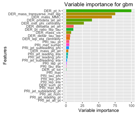
The variable importance graph for the GBM model also highlights the importance of the mass related features, but also the derived momentum as well.
XGBoost
We then used XGBoost to attempt to improve the results achieved thus far. XGBoost is a fast gradient boosting algorithm implementing in C++ by Tianqi Chen. It allows for some parallel computation, more tuning parameters and is generally faster and performs better than gbm; this is due to coding efficiency and the fact that xgboost is not a completely greedy algorithm (unlike gbm).
We also performed a 5-fold cross-validation using a tuning grid, resulting in the following parameters:
- nrounds i.e. number of trees: 200
- max_depth: 5
- colsample_bytree i.e. percent of parameters used at each split: 0.85
- eta i.e. learning rate: 0.2
In summary:
- AUC on training data = .9254
- Kaggle rank = 1340
- AMS = 2.49958
The XGBoost model performed better than GBM but still not as well as Random Forest, for the chosen parameter values.
The variable importance graph for the XGBoost model also highlights the importance of the mass related features.
Step-by-step code used to run XGBoost is shown below:
- Read in the data, perform data munging, create train/test datasets:
- Tune XGBoost parameters by iterating until model stable (1st and 5th tune shown below):
- Use predictions on training dataset to plot ROC-AUC and determine best threshold:
- Predict on test dataset and create submission file for Kaggle:
Ensembling
Finally, we ensembled our 3 models by majority vote in an attempt to further improve the overall model accuracy.
We ultimately achieved a slight improvement on the Random Forest model:
- Kaggle rank = 1309
- AMS = 2.58510
IV. Room for Improvement
As with any modeling, there is always room for improvement. In particular, feature engineering i.e. including additional variables could improve our model's predictive accuracy:
- Introducing basic physics features, e.g. Cartesian coordinates of momentum variables
- Advanced physics: e.g. CAKE variable
- Better understand the physics of additional variables
- Perform appropriate transformations on variables, such as the log transformations described above
In addition, using more machine learning algorithms, more sophisticated ensembling methods and esembling running different random seeds for the same model could further increase the discriminating accuracy of our final model.
In the meantime, if you have any comments, suggestions or insights, please comment below!


