Data Housing Price Predictions Using Advanced Regression
Introduction
When confronted with numerous predictors and a heterogeneous dataset, accurately predicting a response variable can be a non-trivial task. In this article, we outline an approach to feature selection and engineering and machine learning modeling that enabled us to obtain one of the top two Kaggle scores (out of 12 competing groups in the seventeenth NYC Data Science Academy boot camp cohort) in a Kaggle house price prediction competition.
The Dataset and Competition
The Ames Housing Dataset, consisting of 2930 observations of residential properties sold between 2006-2010 in Ames, Iowa, was compiled by Dean de Cock in 2011. A total of 80 predictors--23 nominal, 23 ordinal, 14 discrete, and 20 continuous describe aspects of the residential homes on the market during that period, as well as sale conditions.
In 2016, Kaggle opened a housing price prediction competition, utilizing this dataset. Participants were provided with a training set and test set--consisting of 1460 and 1459 observations, respectively--and requested to submit sale price predictions on the test set. Intended as practice in feature selection/engineering and machine learning modeling, the competition has been unfolding continuously over a nearly three-year span, and no cash prizes have been awarded.
Submissions are evaluated based upon root-means-squared error (RMSE) between the logarithm of the predicted sale price and the logarithm of the actual price on ca. 50% of the test data. As such, the lower the RMSE, the higher the ranking on the competition leaderboard. To date, the public leaderboard consists of 4775 predictions, ranging from RMSE's of 0.01005 to 27.82859, with a median score of 0.13584.
Exploratory Data Analysis (EDA)
In this section, the data preprocessing, data analysis, feature selection, and feature engineering phases of the project are discussed.
Data Preprocessing
Prior to engaging in analysis of dataset trends, lists of each feature type (nominal, ordinal, discrete, and continuous) were constructed by performing regular expression ("regex") searches on a data documentation file associated with the aforementioned de Cock Ames Housing Dataset study.
Outliers
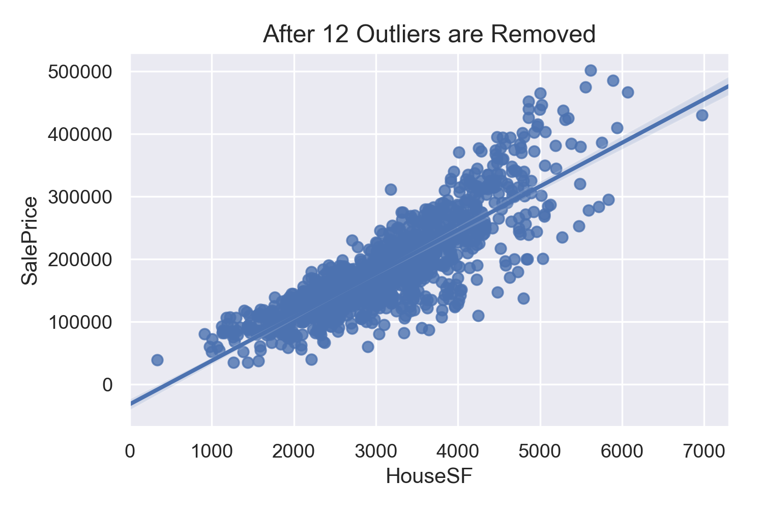
As is indicated in the figures below, 12 outlier observations were removed from the training set after performing simple linear regression on an engineered variable with strong correlation to the response variable (SalePrice):

Response Variable
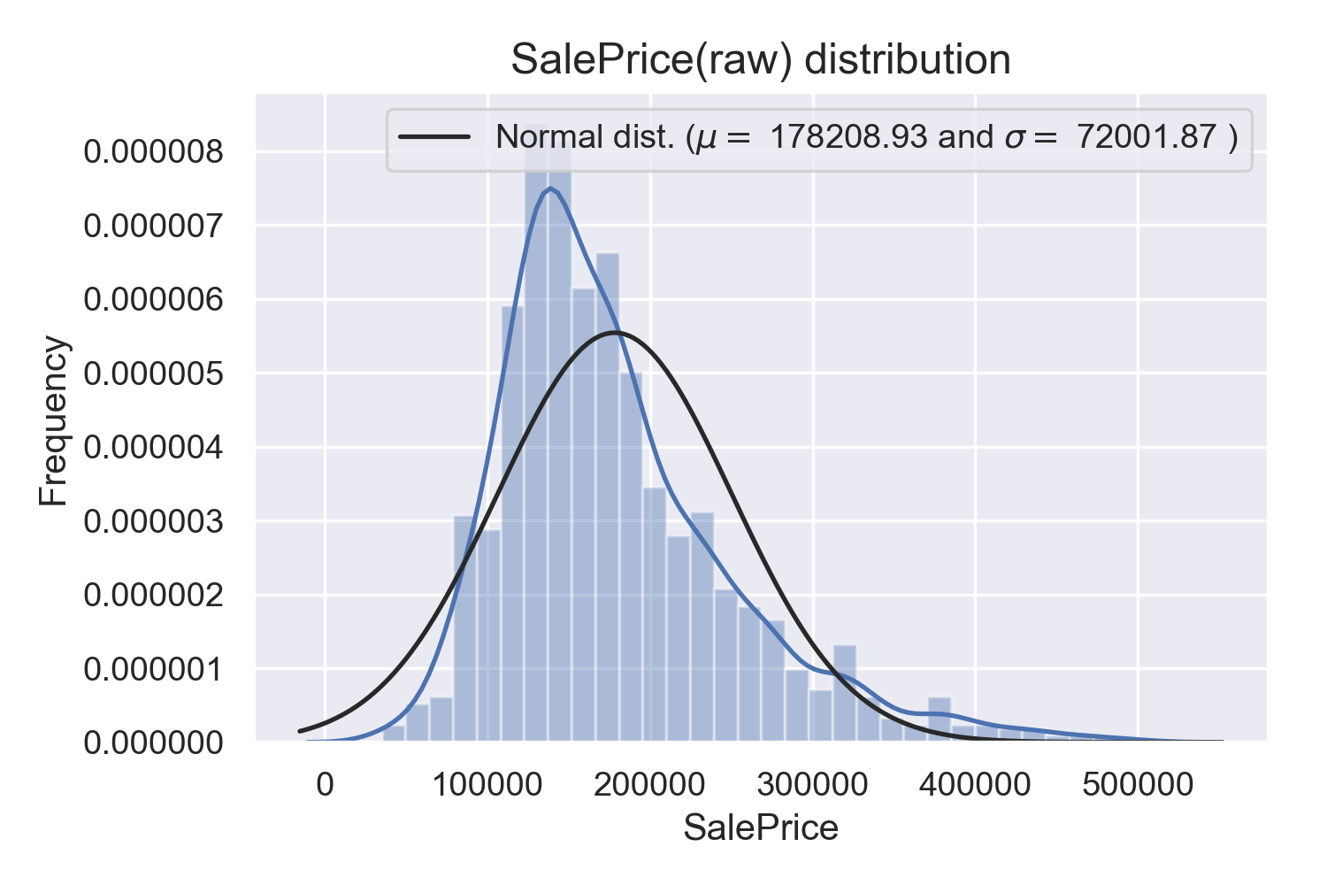
Given that the response variable demonstrates skewness, and that the RMSE for Kaggle submissions is calculated based upon the log predicted price, a log transform was applied to the SalePrice feature in the training set. As a result, the distribution is (sufficiently) normalized:


Exploring Features by Type
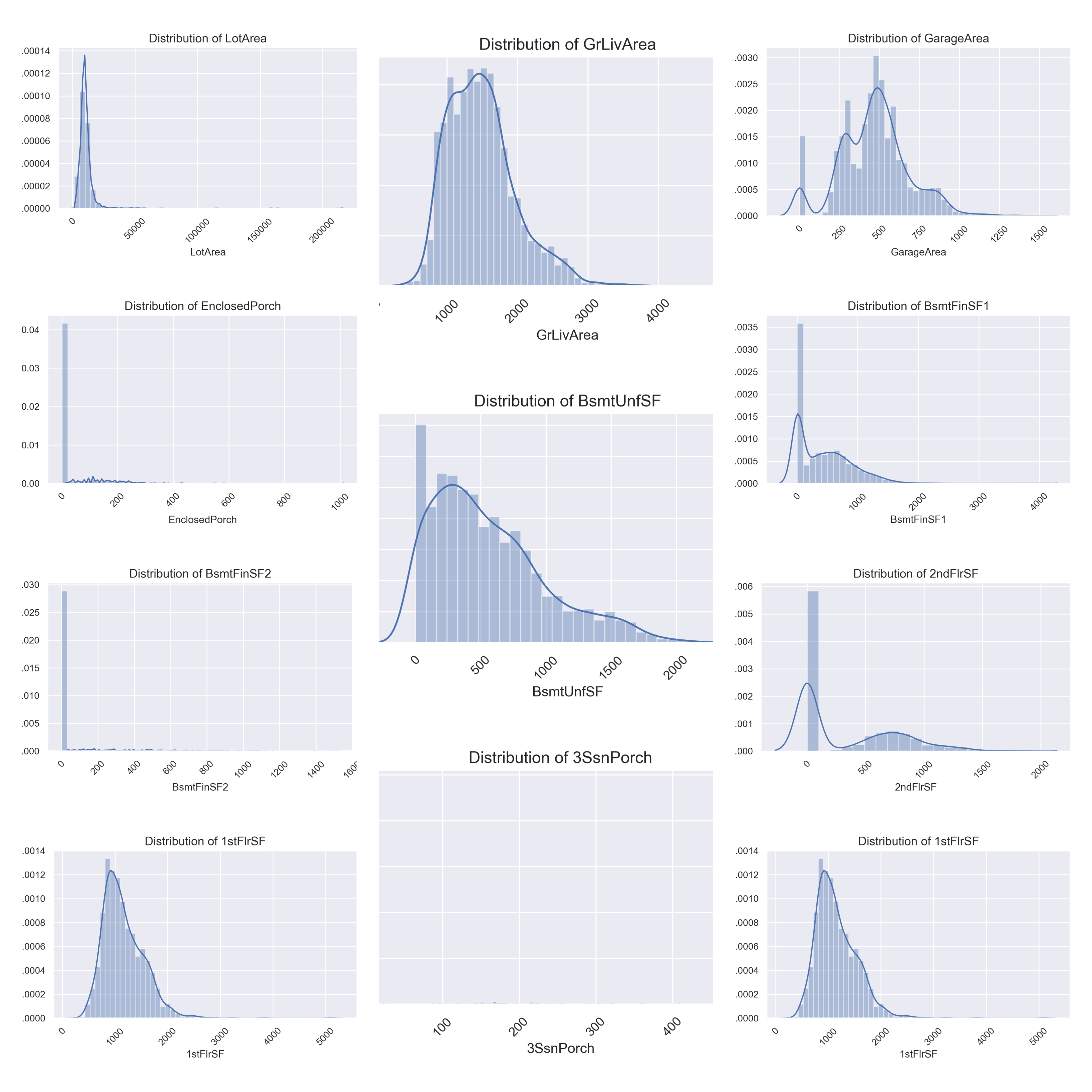
Below are distribution plots of nominal, ordinal, continuous, and discrete variables, respectively. As was the case for the response variable, predictors were investigated for skewness.
Correlation Levels
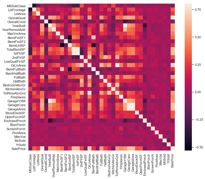
The following heat map visualization indicates levels of correlation amongst continuous variables, and between continuous features and the response variable (SalePrice):
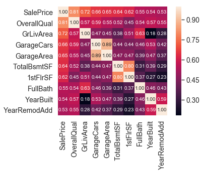
In_the interest of viewing feature relationships at a higher level of resolution, a correlation matrix and pairs plot for the nine predictors most correlated with the SalePrice variable are provided below. (These plots exclude engineered features, which will be discussed later.)

Missing Values and Imputation
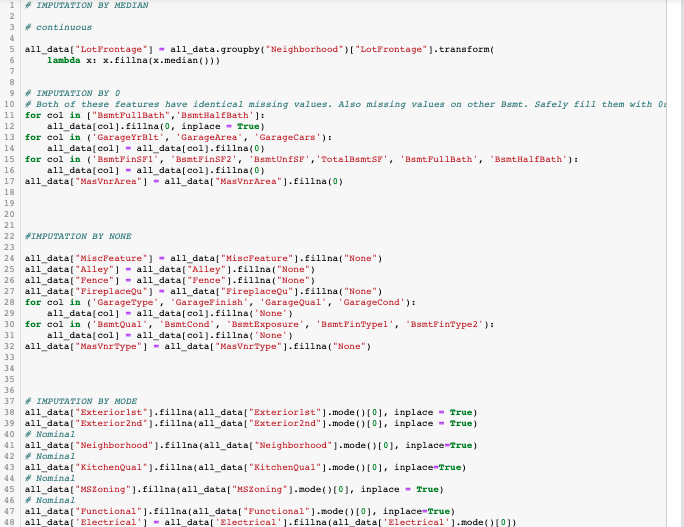
A significant number of columns contained missing values. However, the reasons for and impact, impact, and type of missingness (missing completely at random, missing at random, and missing not at random) varied. As such, it was necessary to carefully apply the appropriate imputation method each relevant feature.

Feature Engineering
Four aggregating features were added to the dataset: Num_Bathrooms (total of all full and 1/2 baths in house), ExtStructSF (total surface area of porches and decks), HouseSF (total interior surface area, as mentioned and utilized in the Data Preprocessing "Outliers" subsection above), and YearRemodAgg, which takes the maximum of YearBuilt and YearRemodAdd.
The YearRemodAgg feature was created with the rationale that a recently remodeled/modified older house would most likely carry greater market value than an unmodified house whose year of origin (YearBuilt) was most recent than that of the remodeled house, but earlier than the older house's remodel date. As illustrated below, YearRemodAgg is strongly correlated to SalePrice:
Nominal Categorical Feature Inspection and Column Dropping
Initially, we took an aggressive approach to dropping columns--especially those of nominal categorical features--that manifested skewness or seemed to be closely correlated with other predictors. However, given improved performance via retaining more features, a more conservative approach was adopted.
As Neighborhood contained the greatest number of factor levels (25 in total), it was instructive to inspect this feature to determine level of variability between and within neighborhoods with respect to sale price:
Given the variability amongst the different neighborhoods, but the relatively narrow IQR's, it was determined that it was crucial to preserve Neighborhood as a predictor.
(This decision was also guided by domain knowledge and research into the Ames housing market. Income levels and other resident and district characteristics vary considerably across the city.)
Ultimately, it was decided that Utilities (which demonstrates 100% skewness) and SaleType (which reflects the buyer, as opposed to a property of the house) would be dropped.
The highly skewed and uninformative Condition2, Heating, RoofMatl (roof material), and Street (gravel or paved access to property) were also deemed dispensable.
Final Preparations for Modeling
Two versions of the dataset were exported to CSV: one in which nominal categorical variables were one-hot encoded (for linear regression purposes), and one lacking one-hot encoding (for tree-based models). The former contained 189 columns, the latter 75.
Machine Learning Modeling
For this project phase, two unique approaches were taken to model testing and selection.
Approach 1: Standard Scaling, Standard Models
In the first, data was scaled using a standard scalar. Simple linear and penalised regression (Ridge and Lasso), as well as random forest, Gradient Boosting (GBM), Support Vector Regression (SVR) (with radial kernel), and a stacked model consisting of Ridge, Random Forest, and GBM components were tested and applied.
From the list of feature importances for GBM, it is evident three of the four engineered features were strongly influential, and that neighborhood was a vital nominal categorical variable. Similar patterns were evident for the Random Forest algorithm.
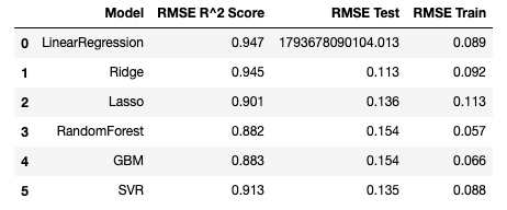
Below are the scores obtained for each model. (N.b.: R^2 Score here refers to training set coefficient of determination.)
Despite the promising low test RMSE's for Ridge and Lasso, the highest obtained Kaggle score was 0.12545. For the stacked model, the lowest test RMSE score was ca. 0.1333. Consequently, a second attempt, using a robust scaler and testing on a broader range of models, was made. In this case, models were grouped into two broad categories: non-ensembling (Linear Regression, Decision Tree, KNN, and SVR) and ensembling (Random Forest, GBM, AdaBoost, and Extra Trees).
Approach 2 Non-Ensembling Models: Linear Regression, Decision Tree, and SVR
In this category, non-regularized linear regression, regularized linear regression (Ridge, Lasso, and Elastic Net), as well as the CART Decision Tree, K Nearest Neighbors (KNN), and Support Vector (SVR) regressors were tested and compared. The box plot below indicates cross-validation mean squared error (MSE) ranges. As was the case for the first approach, Ridge and Lasso gave the best performances:
Approach 2 Ensembling Models: AdaBoost, GBM, Random Forest, Extra Trees
The figure below illustrates MSE rates for the aforementioned ensembling models considered. GBM outperforms other candidates.

Ensembling algorithm comparison. AB = AdaBoost, GBM = Gradient Boost Model, RF= Random Forest, ET = Extra Trees.
Hybrid Weighted Model: Ridge + GBM
Given the above algorithm comparisons, we applied a combined weighted model, with 80% Ridge Regression influence and 20% GBM, as indicated below. This model resulted in the best obtained Kaggle score (thus far).
Final Results: Kaggle Submission
The best obtained Kaggle score was an RMSE of 0.1202. This corresponds to the top 22.3% of submissions to date. In comparison to the 11 other groups competing within the current NYC Data Science Academy cohort, our score was second only to one other team. 
Conclusions
Based upon the outcomes of this project, the following generalizations can be made:
- While removing features with a high degree of skewness may reduce noise in the model, it is preferable to err on the side of caution of too many features than too few, and to enable the models themselves to attenuate overfitting via hyperparameter tuning.
- The four engineered features exhibited high degrees of correlation with the response variable, and proved to be important for both linear regression and tree-based models.
- Among individual models, Ridge Regression and GBM demonstrated superior performance. The optimal results were obtained via a weighted hybrid model of Ridge Regression and GBM.
Future Work
In the interest of further optimizing model performance and exploring the machine learning models applied in this study in greater depth, it would be of interest to:
- experiment with other combinations and quantities of features;
- introduce a larger number of novel features;
- implement a wider palette of stacked models;
- enlarge the Ames dataset (in terms of both number of observations and timespan), and apply EDA and modeling methods to contrasting housing price datasets; and
- streamline the data analysis/transformation processes using a set of functions that could be applied to any comparable labeled data with heterogeneous feature types.
Further Information/Links
Project GitHub Repository || Youngmin (Paul) Cho's LinkedIn Profile || Alexander Sigman's LinkedIn Profile


