LendingClub: Achieving 10%+ Returns with LendingClub
The skills I demoed here can be learned through taking Data Science with Machine Learning bootcamp with NYC Data Science Academy.
Introduction
Founded in 2006, LendingClub rapidly grew to become the world’s largest peer-to-peer lending platform, originating $3bn of loans in 2019.

LendingClub’s business model is to match investors looking to earn returns with borrowers. Both borrowers and lenders are able to get better rates than they would from traditional banks. LendingClub charges borrowers an origination fee on the loans, and a servicing fee on payments made to the lenders. In August 2014, the company raised $1 billion in the largest technology IPO of the year.
Credit Quality on LendingClub’s Platform
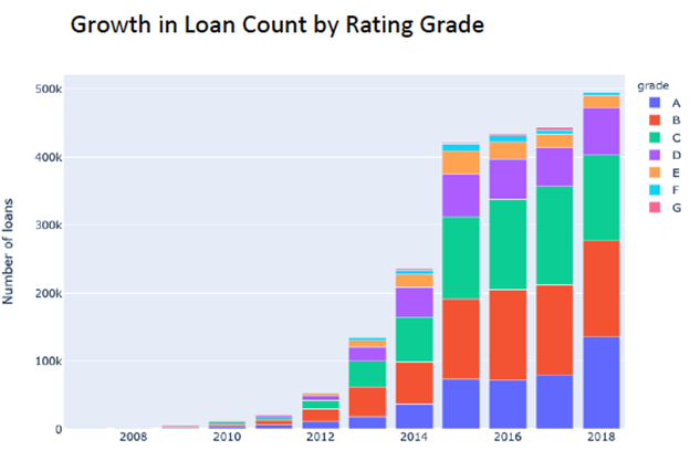
LendingClub initially had 7 major grades of loan rating from A – G. As the company’s issuance volumes grew in 2013 and 2014, the default rates on the two lowest-quality grades increased substantially. This led to investor returns for these ratings becoming negative from 2015 on.

This collapse in investor returns occurred in spite of LendingClub aggressively raising rates on its lower grade loans – highlighting the importance of careful loan selection by investors.

Key Business Questions
Given the wide variation in returns on the LendingClub platform, a potential investor faces three key questions:
- Is it possible to predict which loans will be ‘good’? Defining a precise metric for ‘good’ is part of the required analysis, but clearly non-defaulting loans are preferable to those that do. Also, for non-defaulting loans, those with higher interest rates are clearly preferable.
- How should loans be combined together into an optimized portfolio that diversifies away the risk of any single borrower?
- If we apply the results from our first two questions to a realistic trading strategy, what aggregate returns are possible?
The following sections discuss our analysis of these questions.
Defaults and Random Portfolio Returns
LendingClub makes available all of its historical loan data including 149 pieces of information describing both the borrower (anonymized) and the loan. This loan database spans the entire history of LendingClub and is published quarterly.
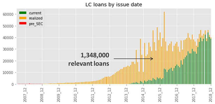
Our specific dataset included all issue dates until December 2018, a total of about 2.3 million loans. We removed about 1 million current loans that had not yet ended either in repayment or default, as well as a few thousand of very old loans issued before LendingClub registered with the SEC.

When the loan originates, LendingClub assigns each loan a grade (A-G) and a subgrade (A1-G5) to reflect the perceived risk of the borrower. All loans eventually end up in one of the 3 categories:
- paid on time
- pre-paid early (no penalty for the borrower)
- default

High default rates are a key challenge for LendingClub and other peer-to-peer lending platforms. For example, the largest subgrade C1 has a default rate of 19%, whereas the traditional consumer credit default rates in the U.S. (e.g. credit cards) are in the range of only 4-5%.
Because the default rate gets so large for lower grades, it pushes down the actual returns for investors. For the higher grades A and B, random investing can produce close to 4% IRR (annualized return), but for the middle and lower grades the performance quickly deteriorates, and starting from grade D it’s already negative.
You lose money if you invest in grade D and below randomly:

So given how bad the defaults are for returns, the question is, can we use the information available when the loans originate to detect those that are likely to default?
Predicting Defaults
When building an actual loan portfolio, we should not simply avoid potential defaults at all cost. Such strategy would produce portfolios consisting only of 4%-bearing A1 loans, and we can do much better than that as we will show below. Therefore, it makes no sense to lump all LendingClub loans in a single training set for the classifier. Instead, each risk category (subgrade) should be analyzed separately.
Predicting potential defaults is a traditional binary classification task, which we approached as follows:
- Remove all features not known at the time of the issue and engineer new features such as the length of credit history and the flag for having a loan description
- Train and test a binary classifier for each subgrade using rolling windows. E.g. use all available data up to 2015 to predict defaults for the loans issued in 2016
- Choose the metrics: precision (lift) for the top predicted probabilities of non-default. We do not care about passing on a good loan (Type II error) because there are about 40,000 new ones issued every month, we care about investing in a bad loan (Type I error)
- Deploy and compare several models including XGBoost and neural networks. The simple 2-layer neural network showed the best performance
The table below summarizes neural network’s top-10% lifts for a few selected subgrades:

Subgraade C1
Using subgrade C1 as an example, random investment into C1 yields 82% of good loans, but the top-10% classified loans would produce 89%!
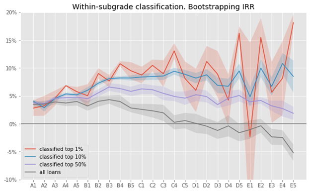
Such reduction in the number of defaults has a very positive effect on the returns across the subgrades. On the chart below, the black line is the uninformed investment return, and the color lines represent consecutive levels of selectivity: top-50%, top-10% and top-1% of the loans:

The annualized returns for such selected portfolios reach 10% IRRs and above. For example, if we apply our classifier to subgrade C4, we could achieve 11-12% IRR.
Given that for most subgrades, there are 1,500-2,000 new loans issued every month, such classification would be equivalent to investing into the best 15-20 loans monthly (within each subgrade). This can accommodate both the retail demand but also some smaller institutional demand such as family offices.
Now that we proved that we can reduce the share of defaults significantly, we decided to build concrete portfolios of LendingClub loans and backtest them in a realistic simulation framework.
Portfolio Construction & Optimization
With a powerful classifier in hand, we proceeded to build tools to intelligently select the best performing loans at the time investment decisions. We then combined them in their optimal proportions to yield the highest portfolio level return given an investor's risk tolerance.
To do this, we first needed to calculate a loan valuation metric that can be used to rank all available loans. To get our feet wet, we started with a simple 1-step approach.
1-step Approach: Present Values
This required calculating the present value (PV) of cash flows for each loan using the appropriate market rate (Fed Funds up to the 5-year US treasury rate) spanning the duration of each cash flow to more realistically calculate each loan's PV and associated internal rate of return (IRR). We then trained a regression model (Gradient Boost Regressor) on the PVs and used the model to predict the PVs of loans in the test set. The highest performing loans ranked by predicted PVs were run through our trading simulator.
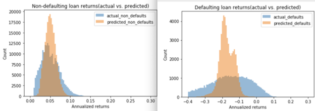
However as seen in the charts below, the distribution of loan PVs is very different between non-defaulting (left) and defaulting (right) loans. This suggests training two separate models, one each for defaulting and non-defaulting loans, may result in more accurate predictions. This led us to explore a 2-step approach.

2-step Approach: Predicted Expected Returns
In the 2-step approach, instead of using PVs, we adopted expected returns as our loan value metric. We fit 2 models: Model_1 was trained on returns for non_defaulting loans in the train set while Model_2 was trained on returns for defaulting loans.
Monthly cash flows were estimated in the same manner as in the 1-step approach with the following assumptions:
- fixed cash flows m, re-invested at a monthly rate r
- cash flows received at monthly intervals [0,n], n= last payment month
- total cash flows are re-invested at r till loan term
With these assumptions, the resulting cash flows form a geometric sequence:

with Total cash flows received given by:

Annualized returns for each loan were then calculated using the total cash flows received shown above as the numerator, the funded amount of each loan as the denominator and r as the fixed re-investment rate of total cash flows received from the last payment date to the term of the loan.
We then weight the return predictions of Model_1 and Model_2 by the relative probabilities from our classifier to get the predicted expected return (R') of each loan in the test set.
Formulaically, we have:

We note however from the graphs below that while the regression model (Random Forest Regressor) did well predicting out of sample returns for non-defaulting loans, it struggled to capture the extreme tails associated with defaults in the defaulting set.

Risk Measures
Each incremental unit of return comes with an associated risk. To quantify this risk, we explored 2 risk measures: Standard Deviation and Expected Shortfall with VAR at the 95% Confidence Level (ES_95).
The training set was grouped by Lending Club's sub-grade buckets and each of the risk measures was calculated using actual returns of loans found within each sub-grade. Each loan in the test set was then assigned a risk measure based on their sub-grade. We also explored K-means clustering as an alternative clustering technique but ultimately settled on sub-grades as these buckets are much more intuitive and more clearly defined.
Measure
While standard deviations are popular in the literature, the measure assumes normality of return distributions but as we can see in the chart below, the returns here are very heavily left-skewed due to defaults violating basic normality assumptions.

Standard deviations if used as a risk measure for this dataset will, therefore, tend to underestimate true downside risk for each sub-grade as shown in the bottom graph.

Consequently, our preferred risk measure for this dataset is the expected shortfall and that's predominantly the risk measure used in our portfolio optimization and analysis.
The top 100 loans sorted by predicted expected returns in the test set were seeded to the optimization routine.
Portfolio Optimization
The purpose of the optimization module is to select the optimal allocation to put to each loan subject to funding and budget constraints that maximize portfolio returns for each level of risk tolerance.
Formulaically we have:

To prove that seeding the optimizer with a set of loans filtered by expected returns informed by the relative probabilities of our classification model resulted in the optimal portfolio, we seeded the optimizer using other filtering schemes, keeping the risk aversion parameter unchanged and compared results. We tried randomly selecting loans in the test set as well as selecting loans with the highest predicted returns regardless of default probabilities amongst other filtering schemes. The table below shows that the expected return filter using our classifier and 2-step regression predictions far outperforms all other metrics across both risk measures.

To more closely simulate a real trading environment, we run the optimization routine on a monthly basis, resulting in optimal monthly portfolios consisting of loans issued that month only and therefore newly available for investment in that particular month. We then ran these monthly optimized portfolios sequentially through our training simulator.
Simulating an Implementable Trading Strategy
A real-world trading strategy on LendingClub faces two challenges. The first is that the predictive model can only use the information available at the time the prediction is made. The second is that the opportunity to invest in a loan exists only for a brief window prior to issuance. For example, we are not able to wait until 2016 and then decide we’d like to purchase a loan from 2012.
In order to address these concerns and test our forecasts more robustly, we implement a trading simulator. We began by fitting our model using an expanded window of returns. That is, we predicted 2014 loans using data from loans that terminated before 2014, and we predicted 2015 loans using the larger dataset available at that time. We continued this way through our entire dataset of completed loans.
We then used these fitted models to select an optimal portfolio of loans each month. For example, we reviewed all the loans originated in January 2014 and selected the 100 best, combining the classifier with the return forecast and portfolio optimizer described above. We introduced some constraints on the tactic, such as the total external funding it was able to draw down ($1 million), and a maximum monthly spend (to avoid it growing the portfolio to fast at the start). Once the tactic had drawn down its maximum amount, loans were purchased only to reinvest cashflows received from the loans in the portfolio.
Baseline
To establish a baseline for comparison, the trading simulator also built portfolio containing the same number of loans for each month, but where the loans were selected completely randomly from all those available. We calculated cashflows for each portfolio and compared the resulting IRRs. The table below summarizes our results.

Overall, our selected portfolio generated cashflows with an IRR of 11.9%, compared to a negative return of 2.9% on the random portfolio. On average, the model selected higher-yielding lower grade loans, resulting in a portfolio with an average rating of D3. It’s notable that the average PV of loans selected substantially outperformed the random portfolio in all three years simulated.
Conclusion and Future Work
We built a tool that can predict the probability of the loan default and its returns for an investor. Based on those predictions we can then construct an optimal portfolio with realistic conditions. It is therefore an end-to-end tool that can be used by both retail and institutional investors in their investments decision.
Simulated out-of-sample returns can reach 10-12%, which makes LendingClub loans an interesting asset to invest!
We also identified several directions that may further improve portfolio performance:
- implement survival analysis approach and more accurately estimate the variance of returns for defaulted loans
- include macroeconomic data such as unemployment rate as external predictors of default probabilities
As a final step, it would be interesting to replicate this analysis on the data provided by Prosper, LendingClub’s closest competitor, which also makes its data publicly available.

