Forecasting the Higgs Boson Signal
Contributed by Denis Nguyen, Kelly Mejia Breton and Ismael Jaime Cruz. They are currently in the NYC Data Science Academy 12 week full-time Data Science Bootcamp program taking place between April 11th to July 1st, 2016. This post is based on their fourth class project - Machine Learning (due on the 8th week of the program).
The Higgs Boson is a type of unstable subatomic particle that breaks down very quickly. Scientist studies the decay of the collision and works backward. To assist scientist in differentiating the background noise from the signal, we offer some machine learning algorithms to better predict the Higgs Boson.
Exploratory Data Analysis
Like all data science projects, we began with some exploratory analysis of the variables.
We first used a correlation plot to inspect the different relationships going on between variables. As indicated by the dark blue and dark red points, there seems to be a high correlation among many of the variables. We noticed the PRI_jet variables, for example, have a lot of blue dots in relation to the variables DER_deltaeta_jet_jet, DER_mass_jet_jet, and DER_prodeta_jet_jet. This is likely since according to the documentation for the challenge, those DER variables are derived quantities computed from the PRI or primitive quantities measured from the particles.
Next, we wanted to zoom in on the correlation plot and see some scatterplots of select variables.
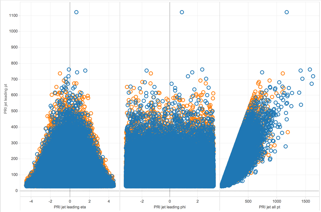
Here, we looked at scatterplots between PRI_jet_leading_pt with the three variables PRI_jet_leading_eta, PRI_jet_leading_phi, and PRI_jet_all_pt. The orange circles represent events that were classified as signal while the blue circles were those classified as background. We noticed some variables seemed to have a linear relationship, such as PRI_jet_leading_pt and PRI_jet_all_pt, while others did not have any obvious form.
Looking at scatter plots amongst select DER variables, we saw a linear relationship to still be present. Between DER_deltaeta_jet_jet and DER_prodeta_jet_jet for example, there was a negative linear relationship.
Finally, we had a look at some scatter plots between a DER variable and a few PRI variables. We found it interesting to see the plot of a DER variable and its related PRI variable from which it was calculated from. For instance, the variable DER_deltaeta_jet_jet and PRI_jet_subleading_eta had a somewhat v-shape as it is derived from the absolute of the difference between that primitive variable and another.
Classification Tree Approach
Classification tree models are great for descriptive purposes. They produce relatively easy regions to trace the process of the model. Although they tend to have a lower prediction accuracy.
Our first basic tree without pruning produced an accuracy of 72% with 3,
398 terminal nodes and an AMS score of 1.132. The right-hand chart displays the number of misclassified observations by terminal nodes, suggesting a tree pruning of about five terminal nodes (where the errors remain flat as the terminal nodes increase). The pruned tree with five terminal nodes returned a lower AMS score of 1.038. After increasing the nodes to 10 the AMS score increased to 1.24.
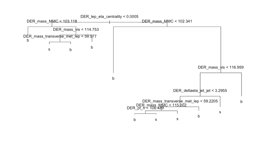
Taking a look at the tree we see the Derived Lep Eta Centrality variable at the very top indicating its importance in determining background noise or a signal of the Higgs Boson. If we were to get a new observation the model would work as follows, beginning at the very top, ask is data point is greater or less than 0.0005? If less go left if greater go right. Moving on to the next terminal node, and so on. Very easy to interpret, but if you are interested in higher predictability this may not be the best option.
Random Forest Approach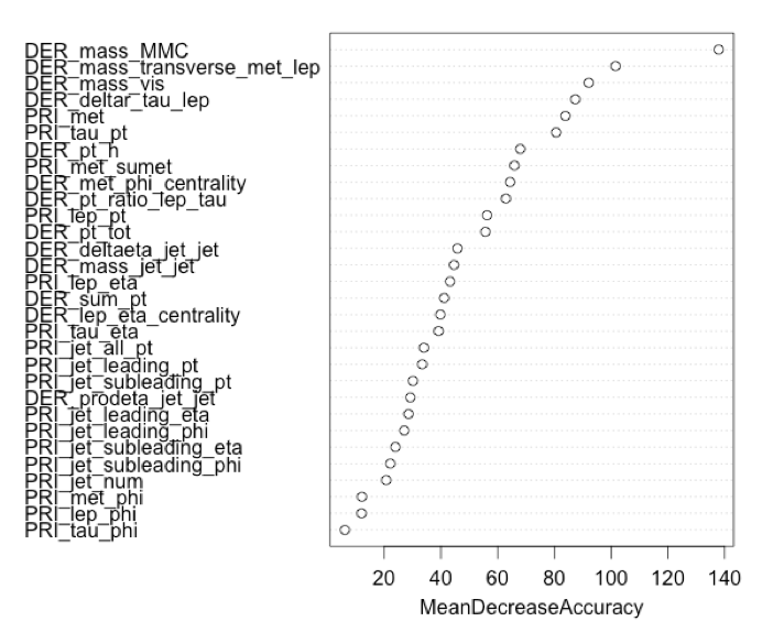
For a more robust model with greater prediction, we attempted a Random Forest. A Random Forest is the average of a collection of trees, resulting in an ensemble with greater predictions. Although, unlike a single tree, you lose descriptive abilities. We ran the model with all the variables, on the right-hand side is the variable importance plot returning an AMS score of 1.781. Impressive, just changing the model type the AMS increased by over 0.5 points.

We then decided to try a model with
only the top 14 variables, along with two columns created to focus on the missing values for DER_mass_transverse_met_lep and DER_deltaeta_jet_jet. We found these columns to individually reduced the errors at most, and together worked great. Resulting in an AMS
score of 2.795 with an accuracy of 83.5% selecting four features at a time at random, creating 500 trees, and taking the ave
rage. This seems like a great model.
Reducing Dimensions
When people think about reducing dimensions, they may think about reducing the amount of information which would result in a less precise model. This is not always the case and it can sometimes improve models. Advantages of reducing dimensions include reducing the time and storage space required, making it easier to visualize data and remove multi-collinearity which would improve the model.
Because there are columns composed of other columns in the dataset, we decided to perform least absolute shrinkage and selection operator (LASSO) to remove possibly related predictors and focus on the ones that would give us a clearer model. After performing LASSO on the variables, we have scaled down many of them down to 0, leaving 12 that we will use.
Gradient Boosting Model
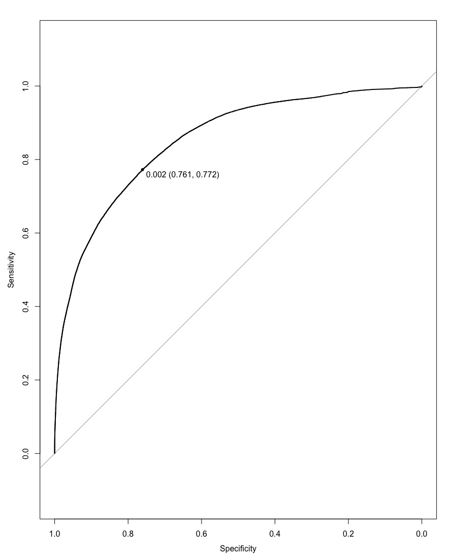
By applying Gradient Boosting Model (GBM) with certain parameters, we were able to get an AUC score of 0.8525 with a threshold of 0.002, yielding an AMS score of 2.28471.
After focusing our model on the 12 variables returned by LASSO, we attained a better score. We got an AUC score of 0.8525 with the same threshold of 0.002. This gave an AMS score of 2.30291, which was higher than the previous model run with all the variables. This shows us that we were able to attain a better predicting model by reducing the number of variables, which probably removed related variables.
Because the AMS score gained was not much higher, we decided to move onto another machine learning method that may yield better results.
Support Vector Machines
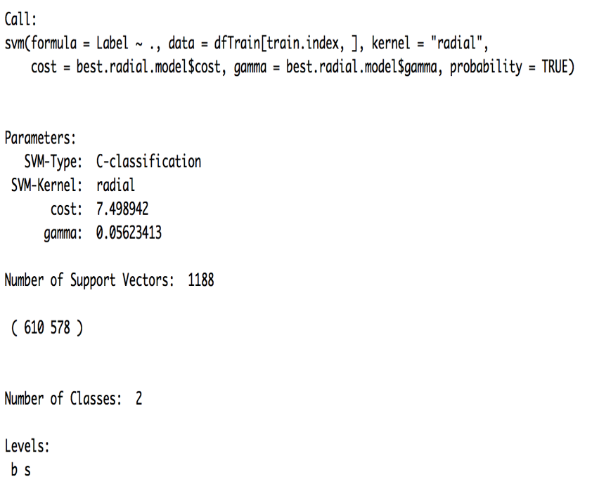
Finally, turning to a more predictive-based model, we attempted using the support vector machine algorithm. Using the scatterplots earlier and seeing as how there was much overlap between signal and background, we chose to use a radial kernel as the problem did not look linearly separable.
The pros and cons of using this algorithm are as follows:
Pros
- Effective in high dimensional spaces
- Choice of kernel
Cons
- Loss of interpretability
- Computationally inefficient when dataset becomes too large
Due to the model being computationally costly with the size of the dataset, we considered tweaking different parameters in order to get it running without consuming too much time. We chose to train it on 1% of the data and used 5-fold cross-validation to find the best estimates for cost and gamma. Next, we used the results from the random forest model and reduced the data set to the 14 most significant variables. Finally, with trial and error, we found the best threshold for the model to be 0.7. Using all these led to an accuracy of 0.8056 and an AMS score of 2.72036.
Recommendation
Considering the number of models we ran for the Higgs boson challenge, we recommend the random forest model since it has the greatest balance of predictability and interpretability. The random forest model gave us the highest AMS score of 2.795 and was able to be trained on all the data. We noted that in terms of AMS score the support vector machine model was second, however, we choose to recommend the random forest model as the latter is less complex to train, has less parameters to tweak, and is not computationally inefficient as the former. In addition, should the main purpose be for description, we recommend the basic classification tree with some pruning.
Next Steps
- Apply some feature engineering to the dataset
- Use ensembling methods to combine the different models that were used


