Decoding the God Particle

1. Introduction

The discovery of the Higgs Boson marks one of the greatest days in science – the standard model had been confirmed. For decades, scientists have searched for the particle that can explain how things have mass, and only recently did ATLAS and CMS experiment begin the building of CERN that lead to this discovery. Following these events, CERN put out a kaggle challenge to test the public’s capabilities in understanding and solving their simulated data.

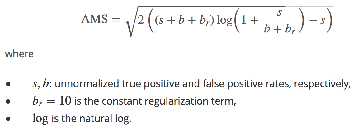
The ultimate goal of the Kaggle competition was to find out machine learning classification methods to improve the statistical significance of the Higgs Boson experiment.  The challenge was designed to develop a model that classified events based on if Higgs boson decays into tau tau channel (signal) or background noise. For this kaggle challenge, team Quark was tasked with creating a two class classification algorithm to determine whether or not an event’s signal is indicative of a Higgs boson’s. Our algorithm was scored based on a metric, called the Approximate Median of Significance (AMS).

The AMS score provided above is a localized formula of the Gaussian significance of discovery - which in its basest form, can be simplified to the ratio of true positives to false positives. Scientists need at least a significance of 5 to make claim to a new discovery, which is equivalent to p = 2.87 x 10-7­­.

The Higgs Boson kaggle dataset was used in this analysis. Exploratory data analyses and algorithm development was performed in R. Our main goal was to maximize the AMS score  - the higher the score, the better our model was able to detect the tau tau decay signal of Higgs boson from known background noise.

2. Exploratory Data Analysis

During the exploratory analysis of data, we noticed that the distribution of variable “weights”, which only appears in the training set, is quite special. When we ranked the weights from large to small in a descending order, we were amazed by seeing that the response variables in the training set could be directly inferred from the values of weights. These findings made us curious about the role of weights in the dataset. It turned out to reflect the true nature of simulation, from which the “signal” only amount to a very tiny fraction of the “background”. The physicist provided more “signal” observation to train the model otherwise what the machine would learn would be basically the pattern of “background” and would not distinguish “signal” and “background” accurately. Therefore, the “signals” typically have lower weight and should be given less emphasis in the model training phase. It seems the weights are a representation of the domain knowledge of the physicist in controlling the price to pay of in the false positive and false negative cases. Based on the data provided, the model is scored higher by predicting “background” correctly than predicting “signal” correctly.

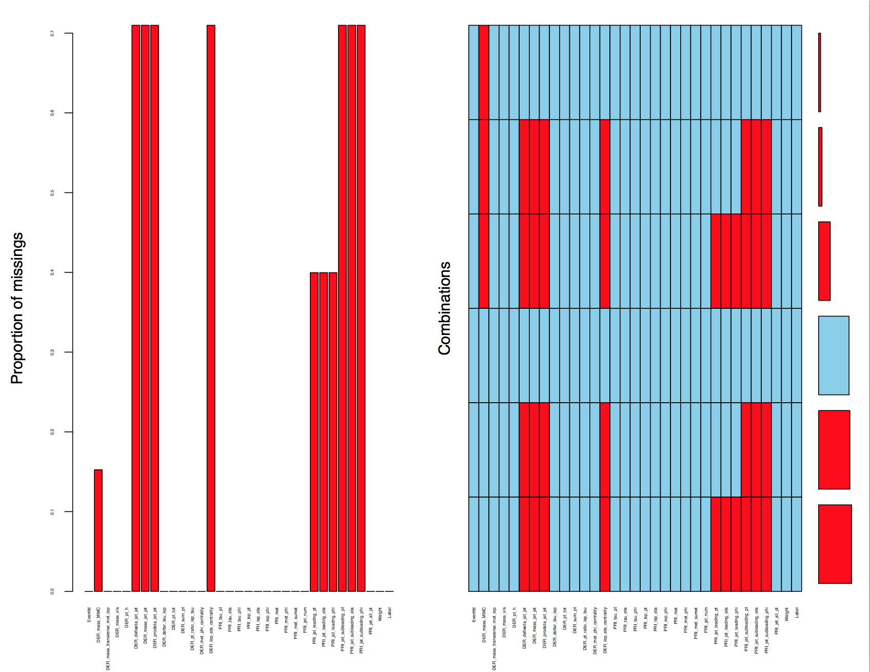
The sheer amount of missing values also caught our attention. We discovered that seven data fields have missing values up to 70% and three data fields have missing values up to 40%. One data field(DER_mass_MMC) has 15.24% missing values. A closer inspection at the pattern of the missingness led us to discover that all missing features are related to PRI jet num except except DER mass MMC. The technical documentation for this competition justified our finding by explicitly stating that some of the features associated with "PRI jet num"(recorded as 0, 1, 2 and 3) are undefined.  

The figure above shows the pattern of the missingness (highlighted in red). We noted from the combinations plot (right side) that there were 6 patterns in our dataset - Only one combination was complete and the remaining five had some missing columns.

For the observations where PRI_jet_num = 0, there were 11 columns with missing values, of which 10 columns were completely missing and “DER_mass_MMC" (The estimated mass of the Higgs boson candidate) occasionally had missing values. Similarly for observations where PRI_jet_num = 1, we found a pattern where there were 7 out of 8 columns values were completely missing and  "DER_mass_MMC" again had occasionally missing values. For the observation with PRI_jet_num = 2 or 3, there were no completely missing columns. The observations all had complete data except for those which likewise, observed "DER_mass_MMC" occasionally missing. It was obvious the features that were completely missing when associated with values of PRI_jet_num are not missing at random (MAR). While we were able to identify the 6 patterns of missingness in our data, we had to ask the question: What is this missingness trying to tell us? Should we be imputing or removing the missing data? Are these columns even necessary?

We then investigated the reason that accounts for the missingness of “DER_mass_MMC”. The visualization of both of the training set and test set helps us to be convinced that the division of observation based on “PRI_jet_num” and missing value pattern could be generalized to the test set. We noticed that the proportion of “DER_mass_MMC” missing value are different across the columns, This tells us that that the % missingness of “DER_mass_MMC” is also not completely missing at random - if it were, we would see equal proportions of missingness across all groups. Interestingly, the proportion of missingness in groups PRI_jet_num in 2 and 3 are similar, suggesting that the mechanism to which their missingness is derived might be the same. One benefit associated with it was that we had more observations to train a single model for PRI_jet_num 2 and 3. Based on our assumption that PRI_jet_num strongly impacts the nature of missingness and should not be treated as a whole, we decided to divide the training and test dataset based on the number of PRI_jet_num values. Given the analysis above, the whole dataset was divided into 3 groups:

Group 1 – Observations with PRI_jet_num value = 0

Group 2 – Observations with PRI_jet_num value = 1

Group 3– Observations with PRI_jet_num value = 2 and 3

After dividing the data into 3 groups, we removed the columns which were completely missing in each group. The documentation provides compelling proof about the reason behind the complete missingness in columns - contextually. It did not make sense for these features to have values; some were specific to multiple jet particles, e.g., variables that ended in _jet_jet meant it was a derived calculation between at least two jet particles. As a result, it was explicitly stated that for PRI_jet_num values below the required value could not be calculated, and as a result undefined. Therefore, it is justifiable to remove the columns that were completely missing in each group. After removing all columns that were completely missing in each group, the only variable that still had missingness was "DER_mass_MMC". The missing data for DER_mass_MMC was unrelated to number of jets due to the topology of the event being too different from the expected topology. As we earlier determined, “DER_mass_MMC” is also not missing completely at random (MCAR), and therefore would not be wise to just remove. In order to ensure we were not removing an important feature, “DER_mass_MMC" required imputation.

3. Imputing the Missing Value in Higgs Mass

To best assess our imputation method, we wanted to check if this variable had any linear relationship with other variables. We plotted a correlation plot for the table with PRI_jet_num = 0, and found that some of the variable were highly correlated with “DER_mass_MMC". Similarly, we found that “DER_mass_MMC" was highly correlated with other variables for groups with jet number one and greater than one. Based on this information, we performed imputation using MICE function.

The missing data in “DER_mass_MMC" for each group was imputed using the Multivariate Imputation by Chained Equations (MICE) function from the MICE package. The function used a Multiple Imputation (MI) approach which is based on repeated simulation; it has been commonly used for complex missing value problems. The function returned a set of complete datasets (by default 5) that is generated from an existing dataset containing missing values. In our case, 5 complete datasets were created by imputing values for “DER_mass_MMC”, by interpreting missing values from all other variables in the dataset for each group using multivariate linear regression. Standard statistical methods were applied to each of the simulated datasets by this function. The final step in imputation for each group was the average of the 5 datasets that were created by the function.

4. Machine Learning Approaches

We used different machines learning approaches to build models, classifying the tau tau decay signal of the Higgs boson from background noise. The models selected were Logistic Regression, Random Forest and Gradient Boosting Machine - the reasoning will be described in the following sections. The models were trained on the training dataset and scored on testing dataset to obtain a final prediction. We then checked the performance of each model by comparing AMS scores evaluated through kaggle submissions.

4.1 Logistic Regression

The first model we decided to try to model the events was Logistic Regression. Logistic regression’s main strengths are its quick training and computation, as well as clear interpretability. Although being a supervised modeling method, it also contains descriptive information regarding the feature selection. Logistic regression is a non-linear log transformation on the traditional linear regression to the odds ratio. As a result, it is a simple and effective method to model classification problems. The assumptions made in linear regression do not transfer over:

1. No assumption of a linear relationship between the dependent and independent variables - only linearity of independent variables and the log odds
2. Error terms do not need to be normally distributed; however they need to be independent
3. No need for homoscedasticity (constant variance)

The results above compare regressions between two models within one group: with and without weights. We wanted to observe the effect of weights. The default threshold value is 0.5 here.The model in the left with weights taken into account has a significantly lower (64% vs 71%) accuracy, nonetheless the highest AMS. It’s reasonable because the evaluation is based on AMS with weights rather than just accuracy. As a result of weights not equally assigned for “signal” and “background, accuracy could be compromised in order to get a higher AMS score in the model training. We could see the prediction of the model favored the “background”, which was consistent with the conclusion we made before.  

The model suggest that DER_mass_MMC is not actually important - the most important being DER_mass_transverse_met_lep, DER_mass_vis, DER_deltar_tau_lep, and DER_pt_ratio_lep_tau. However, based on the previous analysis, DER_mass_MMC is what we expected to be important in determining the response variable. It might be the case that DER_mass_MMC and probabilities for the classification are not linear. We need more proof from tree-based method, which are a group of non-linear methods.

After submitting and scoring against the test set, we got a result of 2.034

4.2 Random Forest

Random Forest (RF) is an ensemble learning method for classification and regression. By creating a large number of decision trees it collates individual trees’ votes in order to predict the class; Sometimes that may be the mode of the classes (classification) or mean prediction (regression) of the individual trees.

4.2.1 Cross Validation

For our Random Forest and Boosting model, we performed “Leave group out Cross Validation(LGOCV)”  or “Monte Carlo cross-validation" to cross validate our training model. Cross validation is an important method to evaluate our training model before it is used against a test set. Traditionally, data sets are split ~70% training: 30% testing and scored. However, not all of the data is used in training and as a result may not improve accuracy. K-fold cross validation, is a method where the whole data set is split among K sets, and K models are trained across K-1 training sets and 1 testing set. It is the simplest method to use, but it only explores a few possible ways that our data could have been partitioned. K-fold cross validation is a good unbiased estimator of the algorithm’s performance, but with high variance. LGOCV allows for further exploration by randomly sampling our dataset multiple times for training sets (25 resamples for our model). LGOCV reduces accuracy variation between the models, at the cost of some bias.

We needed to tune the number of randomly selected features (mtry) used in a given decision tree. For classification problems, it is recommended in “Applied Predictive Modelling” book by author Max Kuhn and Kjell Johnson to start with an mtry values around the square root of the number of predictors. The book also suggested to start with an ensemble of 1,000 trees and to increase that number if performance is not yet close to a plateau to get optimal results. The tuning parameters set for the random forest model for all groups are mentioned in the table below.

The final mtry values for our groupings of PRI_jet_num = 0, = 1, > 1 were 5, 5 and 4 respectively.

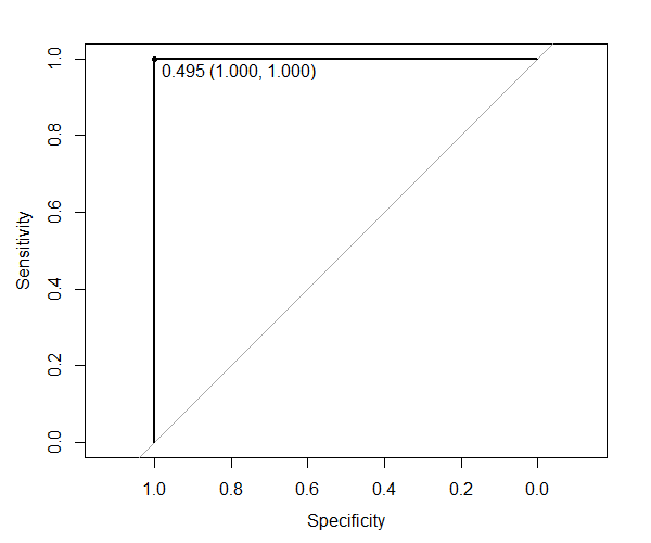
ROC curve (Jet number = 0)

The ROC curves give us information about the threshold value to choose to have the best true positive rate and minimize the false positive rate. For the dataset where PRI_jet_num = 0, we found that the model is able to predict the training observation perfectly when selecting a threshold of 0.495.

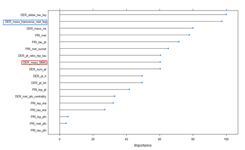
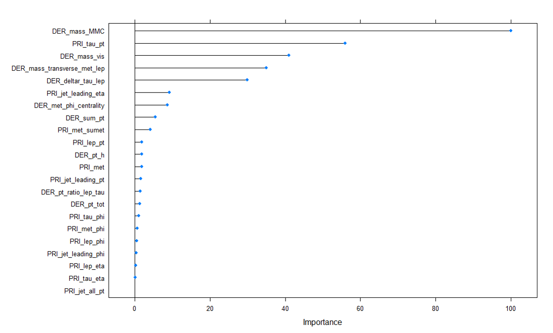
Variance Important Plot (Jet number = 0)

The variable importance graph above for the RF model shows the features that were important for this model. From the plot, we can see that DER_deltar_tau_lep and DER_mass_transverse_met_lep were the two most important features for the model. It was interesting to see DER_mass_MMC ranked 6^th in the variable importance.

ROC curve (Jet number = 1)

For the dataset where PRI_jet_num = 1, we found that the model is able to predict the training set perfectly at a threshold of 0.501.

Variance Important Plot (Jet number = 1)

From the plot, we can see that DER_mass_MMC was the most important variable followed by DER_mass_transverse_met_lep and Der_met_phi_centrality.

ROC curve (Jet number = 2 and 3)

For the dataset where PRI_jet_num > 1, we found that the model is able to predict the training observation perfectly at a threshold of 0.502.

Variance Important Plot (Jet number = 2 and 3)

From the plot, we can see that DER_mass_MMC was the most important variable followed by DER_delta_eta_jet_jet and DER_deltar_tau_lep.  DER_mass_transverse_met_lep moved further down in the importance ranking.

Analyzing variance importance plot for each group, we found that variable importance varied for each group. The dataset that had PRI_jet_num =1 and PRI_jet_num >1 had DER_mass_MMC as the most important variable. However, this was not the case for the dataset having PRI_jet_num = 0; DER_mass_MMC ranked at 6^th   variable importance plot. Therefore this suggests that it is good to have different random forest models for each group because the importance of the variables differed. In all Random forest models, mass was an important feature and is in agreement with the science behind Higgs Boson detection.

Each model and threshold value was used to predict the test dataset for each corresponding group. After predicting the label for the test data set  from each model, we combined data sets for each jet number into one complete dataset and tested for AMS score as instructed in the Kaggle website. The final AMS score achieved by Random Forest model was 2.328, outside the top 50% of the Kaggle leaderboard.

4.3 Boosting

After looking at the results from random forest, the next model that naturally followed was boosting. Random forest is a bagging method, while Boosting works by ensembling many weak learners (shallow decision trees) accounting for small subsets of the total observations. Boosting generally has more predictive power than traditional prediction methods - however, it is not without its flaws: it is significantly more computationally expensive than random forest, there are more parameters to tune, and a higher risk of overfitting.

We trained our boosting model with the following parameters:

Shrinkage is a parameter where the lower the better - it is the learning rate where the errors of one split is understood by the following. We chose a value of 0.001 as it is a decently low value while not being too computationally expensive.

Interaction depth is the number of splits per tree. The maximum interaction depth is defined by the square root of the total number of features (in our case, 32). To be thorough, we tested 1, 3, and 5.

For the number of trees, we continued using the heuristic from random forest i.e., 1000 trees for consistency. However, in hindsight this is a parameter we should have also tuned with a range. Boosting is much more prone to overfitting, and by plotting the accuracy vs. number of trees we would have been able to see the point where more trees no longer gave us better results.

Min Observations is the number of observations taken into account per split. If improperly tuned, this parameter is often what results in overfitting.

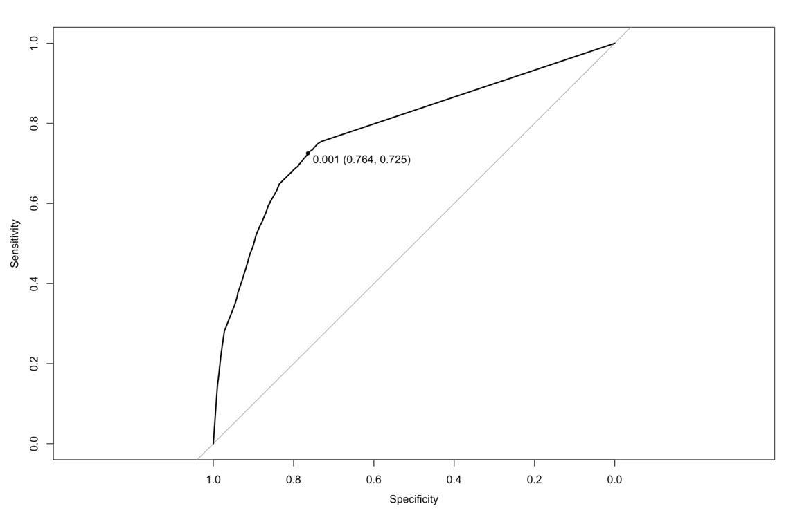
ROC curve (Jet number = 0)

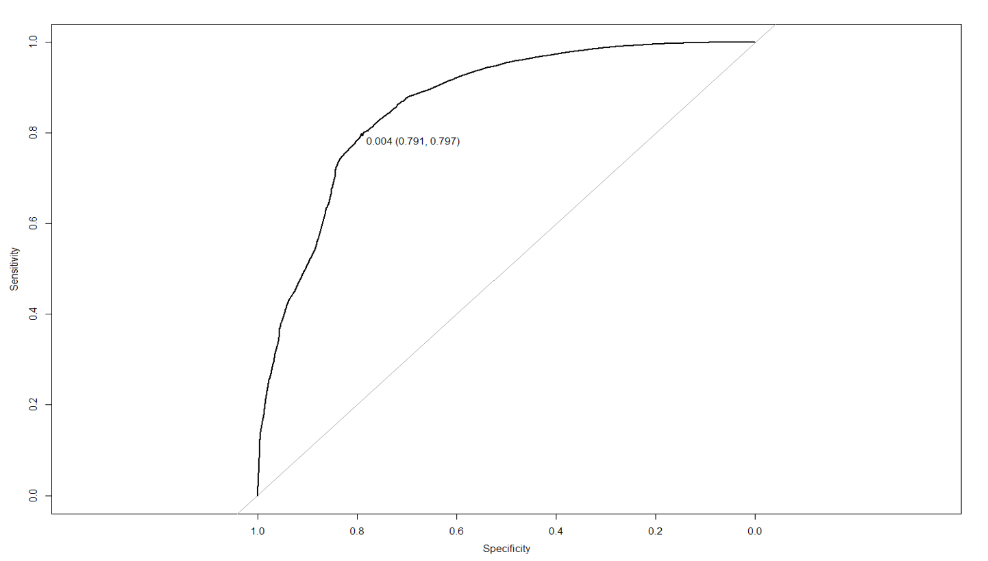
ROC curve (Jet number = 1)

ROC curve (Jet number = 2 and 3)

The above ROC curves detail not only the respective cut off values we chose, but also the resulting tuning parameters for each PRI_jet_num subset. The min obs chose for each model was 100, and the highest interaction depth (5). The only exception was the boosting model where PRI_jet_num = 0. It instead chose only an interaction depth of 1, and perhaps we could see what had happened in the variable importance graph:

Variance Important Plot (Jet number = 0)

Variance Important Plot (Jet number = 1)

Variance Important Plot (Jet number = 2 and 3)

The most noticeable thing is how the varImp graph for PRI_jet_num = 0 hardly took any other variable into account other than DER_mass_tranvserse_met_lep. This makes sense when in context of an interaction depth of 1 (each tree only made a split on one variable that would reduce the gini impurity). Because boosting is greedy, it kept reusing the same variable. This implies that perhaps boosting is not the best method for this subset of data. The final AMS score is a terrible 1.4, which is to be expected.

5. Conclusion

Imputation is just another layer of modeling and should be treated very carefully. It’s like a regression model inside a classification model in this case. If inappropriately treated, it might introduce significant bias in the model and add uncertainty. To make a less biased imputation, it’s critical to understand why the data is missing and if the pattern of missing data is related to the outcome. We were doing well in this regard. Based on our assumption, the whole dataset was divided into three groups and imputed, creating separate machine learning algorithms for each. The predictive models were also scored  separately based on “PRI jet num”.

It’s a bitter lesson to know the AMS scores were not desirable for each algorithm,  especially when compared with the results of our peers. It’s evident that the predictive power of models trained on separate “PRI jet num” groupings were no match for complex boosting algorithms treating the dataset as whole. One possible explanation is that by dividing the dataset into three groups, we essentially cut off the intertwining relationships between the three subset of data and hence lost some degree of predictive power. We assumed that the  “PRI jet num” variable would be so important as to consider the effect of it to the response variable separately. Even worse, after the division the patterned missing values for the two groups ( “PRI jet num” =  0 or 1) became impossible to be kept in the vector space and were removed.  Again, it resulted in loss of information because our separate models had fewer observations to train, to be  generalized,  and to have fewer predictors predicting the outcome accurately.

We finally realized that those patterned missing values, though meaningless to impute in the setting of physics, are instructional on their own. Ironically, it turned out the missing value pattern is exactly one of the most important pieces of information to infer the response variables. One better practice is to potentially code those patterned missing value 0, indicating the fact that they are undefined while keeping the pattern of these reasonably imputed values in the whole dataset. Then each of the distinct classification algorithms, like logistic regression, random forest,etc., could be applied on the whole dataset to learn the patterns, namely, the explicit missingness that sophisticated physicists left there. Without domain knowledge, it’s really important to not let the machine to learn our bias, which was regarding “PRI jet num” in this project. However, we wouldn’t know the result of the prediction unless we tried. Trial and error, that’s how the machine learns and also how we learn.

Link to the code :https://github.com/nycdatasci/bootcamp006_project/tree/master/Project4-MachineLearning/Quarks_Kaggle