Higgs Boson Machine Learning Challenge
Contributed by (Emma) Jielei Zhu, Le Wei, Shuheng Li, Shuye Han and Yunrou Gong. They are currently in the NYC Data Science Academy 12-week full time Data Science Bootcamp program taking place from July 5th to September 23rd, 2016. This post is based on their fourth project - Machine Learning (due on the 8th week of the program).
Content
- Introduction
- 1.1 Background Review
- 1.2 Project Objective
- Methodology
- Pre-processing Data
- 3.1 Subset Data by number of jets
- 3.2 Imputation Missing Value
- Data Description
- Exploratory Data Analysis
- Principle Component Analysis
- Machine Learning Approaches
- 5.1 Random Forests
- 5.2 Gradient Boosting Machine
- 5.3 XGBoost
- 5.4 Reduced Features
- Conclusion
1. Introduction
1.1 Background Review
The discovery of Higgs Boson is crucial, as is the final ingredient of the Standard Model of particle physics, a field filled with physicists dedicated to reducing our complicated universe to its most basic building blocks. The discovery of Higgs Boson was announced on July 4, 2012 and was acknowledged by the 2013 Nobel prize in physics. However, discovery is only the very first step. We still need to understand how it behaves. As it turns out, it is quite difficult to measure the new particle's characteristics and determine if it fits the current model of nature. A key finding from ATLAS experiment is that the Higgs boson decays into tau tau channel, but this decay is a small signal buried in background noise.
1.2 Project Objective
The goal of this Machine Learning Challenge is to improve on the discovery significance of the tau tau decay signal. Using simulated data with features characterizing events detected by ATLAS, our task is to classify events into "tau tau decay of a Higgs boson" or "background".
The data contains a training set with signal/background labels and with weights, a test set (without labels and weights), and a formal evaluation metric representing an approximation of the median significance (AMS) of the counting test. The performance of the classification result is thus evaluated by the following formula:

In sum, the goal of this project is to maximum the AMS score to improve the discovery significance of the tau tau decay signal of Higgs Boson from background noise.
2. Methodology
We first tried unsupervised learning methods to analyze the features of training and test dataset. Secondly, we used different supervised Machine Learning approaches to build models to classify events into either the tau tau decay signal of Higgs Boson or background noise.
3. Pre-Processing Data
3.1 Subset Data by number of jets
According to the description of the features in the technical document provided by the host of this challenge, the "PRI jet num" feature is the number of jets taking on integer values of 0,1,2 and 3. This feature is very unique in that it directly affects missingness in other features (e.g. "DER delta eta jet jet", "DER mass jet jet", and "DER prod eta jet jet" are undefined if the number of jet is 0 or 1). In light of this characteristic of the data, we broke the training dataset into 4 subsets according to the jet number column(i.e. 0, 1, 2 or 3) and then examined the missingness patterns for each subset (below).


From the figures above, we can see that for the 'jet=0' subset, there are 11 columns containing missing values with 10 of them being entirely missing. For the 'jet=1' subset, there are 8 columns containing missing values with 7 of them being entirely missing. Lastly, for the 'jet=2' and 'jet=3' subsets, they have the same pattern of missingness: only the first variable "DER_mass_MMC" contains missing values.
The reason why some of the columns are entirely missing is because the values of these columns are undefined for certain jet number groups. Therefore we deemed it reasonable to drop these columns that are entirely missing. Observing that 'jet=2' and 'jet=3' subsets have the same pattern of missingness, we combined these two subsets, resulting a total of 3 subset, which were 'jet=0', 'jet=1', 'jet=2/3'.
After removing the entire missing value columns, there is only one variable––"DER_mass_MMC"––that still contains missing values. We conducted a clustering analysis on each of the subsets to check whether we should separate the subsets into two groups based on whether the value of "DER_mass_MMC" is missing or not. The result showed out that two groups were not significantly different from each other, suggesting they do not need to treated separately.
Finally, the last step we did with the number of jets feature was to separate the test data into 3 subsets in the same way as we separated the training data.
3.2 Imputation of missing values
After subsetting the training dataset into 3 subsets, only the "DER_mass_MMC" feature still contains missing values (26%, 10% and 6%, respectively). Because the missing percentages are reasonably low, we thought of dropping these observations completely. However, we saw the test dataset also contained observations with missing "DER_mass_MMC" feature, and we can't drop any observation in the test dataset, obviously. So we kept the observations with missing values in the training set, and ended up imputing those values.
To impute the missing values in the "DER_mass_MMC" column, we tried a total of 4 imputation methods:
- PMM(predictive mean matching)
- Random Sampling
- KNN (K nearest neighbors) with varying K's (total of 6)
- Random Forest
To find the best imputation method, we used observations in the training set that had no missing values and took out some of the "DER_mass_MMC" values randomly. We then had each method impute these "artificial missing values". Using cross validation with the "ground truth" labels, Random Forest gave the best result. Thus, we used Random Forest to impute the "DER_mass_MMC" values for both the training and test set (separately for training and test and separately for each subset).
4.Data Description
4.1 Graphical Data Analysis
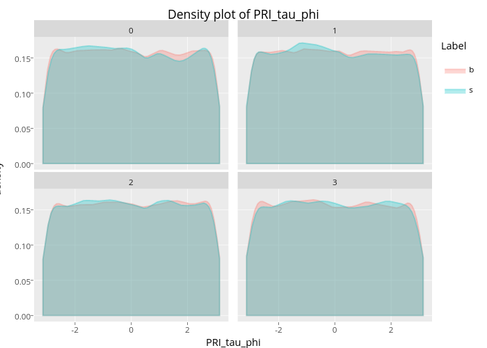
To understand each feature of this dataset, we visualized univariate distributions for each feature. We found that the features whose names end with 'phi' have a uniform pattern as shown from the graph above (plot shown from 'PRI_tai_phi'). The distributions for each class ('signal' and 'background') are extremely alike––nearly completely on top of each other. What this means is that the univariate distribution of the variables whose name ends with 'phi' do not contain much information to help distinguish 'signal' from 'background noise'.
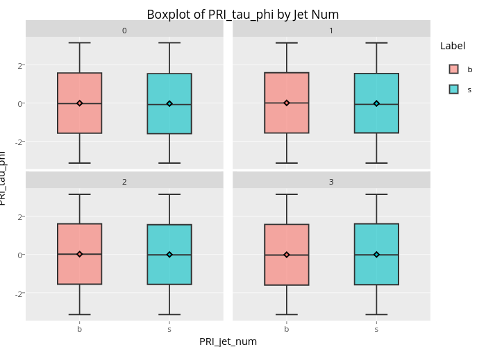
From the bot plot of 'PRI_tai_phi' (see below), we can further understand that the 'phi' type variable is an angle basically, range from -180 degree(-3.14) to 180 degree(3.14) . The distribution is perfectly symmetric and no outliers and no difference by the labels.
However, the identical distributions should never be the reason for excluding these 'phi' features from applying to the machine learning models later on, because they may potentially has great influence for classifying the signal when they combine with other features.
Another important finding from the correlation matrix graphs in each of the subsets is that some of the features are strongly positive correlated to other variables, which may incur multicollinearity problems,
especially for conducting logistic regression models to classify the labels. Thus, we will not perform logistic regression in the following modeling part.
Additionally, 99% of the values of 'DER_pt_tot' are the same as of 'DER_pt_h' in subset data of jet number 0 , which indicates that for further modeling part, we could remove one of the features.In our reduced model part, we dropped the variable 'DER_pt_tot'.


4.2 Principle Component Analysis
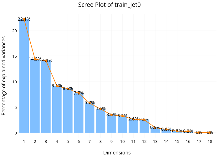
From the Principle Component Analysis(PCA) scree plot for 'jet=0' subset, we found that the first dimension explains about 22.1% of total variance, the second dimension explains about 14.3%, and the third dimension explains about 14,1%. This means the first 3 dimensions together explains only about 50% of the total variance, which is quite low. Additionally, we don't see any sharp drop off in the percentage of variance explained from this scree plot, suggesting no natural cut off point in keeping certain dimensions and discarding others.
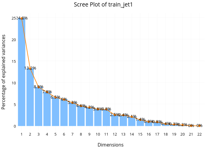
Looking at the scree plot for 'jet=1' subset, we see a very similar pattern––low variance explained for the first few dimensions and no sharp drop off for the later dimensions.
Again, the same pattern for the 'jet=2/3' subset.
From the variables factor map-PCA for train_jet0, we can see that DER_sum_pt, Der_mass_MMC, Der_mass_vis, and PRI_lep_pt contribute almost 80% of their variance on the PCA 1 and also contributed some variance on dimension 2, but not as much as the dimension 1. For dimension 2, we can see that Der_mass_transverse_met_lep contribute almost 80% of their variance on dimension 2, and also some portion of variance on Dimension 1.

From the Variables factor map- PCA for train_jet1, the Der_sum_p contribute a lot of variance on Dim1. For dimension 2, Der_mass_MMC and Der_mass_vis contribute a lot on dim 2, and also contribute part of variance on Dimension 1.
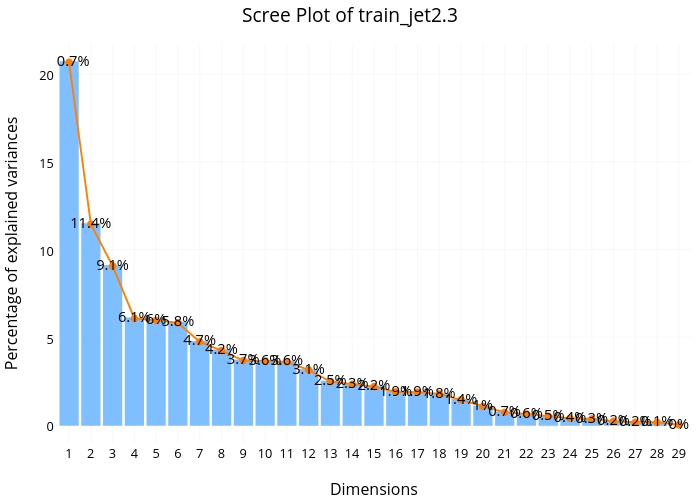
From the variables Factors map-PCA for train_jet 2.3. The Der_mass_jet_jet and DER deltaeta_jet_jet have large portion of variance contributed to dimension one. The variable Der_pt_h, PRi-jet-loading_R have large variance contributed on Dim2.

From the Exploratory Data Analysis on the previous three PCA, we found out that DER_mass_MMC contributed variance a lot on both train_jet0 and train_jet1, so we may assume that this variable has large impact on the total data. But we may use later test to see if this factor is truly important.
5. Machine Learning Approaches
5.1 Random Forest
We tried Random Forest as our first algorithm. We wanted to set a benchmark score and look at which variables Random Forest thinks are important and which are not. Additionally, we wanted to compare and contrast the list of variables PCA thinks are important against the list Random Forest thinks are important. We believed that this analysis would not only let us understand the variables better, it would also help us eliminate some unnecessary variables that contribute little to the AMS score. There were a few variables that we specifically paid attention to, including “DER_mass_lep”—the only variable that contained missing values after segregating data by jet number, and variables that contained the term ’phi’— variables that explain little variance according to PCA.
Our entire modeling process with Random Forest came in 3 stages, with increasing AMS score for each stage (3.28 -> 3.42)
In the first stage, we fitted a Random Forest model for each of the 3 subsets using the ‘rf’ method in the caret package. The best models were selected based on absolute AMS scores, which happened when ‘mtry’ was 20 for each of the subsets (20 was the maximum number tested because . What that means is that the best models all wanted the maximum number of variables for consideration at each splitting point of the tree. The models looked fine, but when we plotted the Receiver-Operating Curve (ROC), we saw the predictions were 100% correct on the training set. This is a clear sign that we were probably overfitting our training data.
To solve, or at least alleviate, the overfitting problem, instead of choosing the models that outputted the highest AMS score, we went after the simplest models that were within 1 standard error of the best empirical models, which brought us to stage 2 of fitting Random Forest models. Using this new selection metric, we picked models that either had ‘mtry’ equals 1 or ‘mtry’ equals 2. When we plotted the ROC again, sadly, we still see a perfect classification rate.
We first fitted a Random Forest model with varying 'mtry' values. The ones tested initially included 1, 2, 5, 20. Out of these values, 20 gave the best AMS scores on each subset, although with marginal differences. We visualized the performance of the best models by plotting ROC and calculating the area under the curve (AUC) score. What we found was a plot that claimed the model was able to predict the training observations perfectly.

AMS = 3.28

How did we find the threshold ?

AMS = 3.42
mtry for 'jet=0' : 1
mtry for 'jet=1' : 3
mtry for 'jet=2/3' : 3
5.2 Gradient Boosting Machine

AMS = 3.35
5.3 XGBoost

ROC Curve for 'jet=2/3' subset

AMS = 3.48
5.4 Reduced Features

6. Conclusion