Machine Learning Kaggle Competition-Mission Zillow

[All authors contributed equally to this blog]

1 Overview

In the year 1959, Arthur Samuel, a pioneer in the field of Machine Learning, defined it as a field of study that gives computers the ability to learn without being explicitly programmed [1]. According to Professor Tom Mitchell at Carnegie Mellon, the field of Machine Learning seeks to answer the following question: “How can we build computer systems that automatically improve with experience, and what are the fundamental laws that govern all learning processes?”

Machine Learning algorithms are broadly classified as supervised, unsupervised and reinforcement learning. In particular, supervised learning algorithms have been used to make predictions based on certain given inputs in a variety of applications. For instance, Zillow revolutionized the landscape of the real estate industry by introducing Zestimate; it could predict the sale price of properties with an accuracy of about 95 %. With an objective to improve the accuracy further, Zillow launched a competition on Kaggle that challenged the Data Science community to develop algorithms that can potentially outperform Zestimate. The competition is phased in two rounds and the objective of the first round is to predict the logerror defined as follows:

logerror=log(Zestimate)−log(SalePrice)

Team Entropy’s approach to this challenge included Exploratory Data Analysis (EDA), Data Imputation and the implementation of a slew of Machine Learning algorithms (Logic based methods, Elastic net regularization (Ridge and Lasso), Tree based models (Gradient Boosting Machine, Random Forest, Extreme Gradient Boosting) and Automatic Machine Learning (h2o) and will be discussed in detail in the subsequent sections.

2 EDA: Analysis of Missing Data

The team started EDA by looking at the missingness in the dataframe. Knowledge on the nature of missingness allowed the team to make plans for subsequent data imputation. The degree of missingness is shown in the plot below. Figure 2 shows that most of the variables have certain degree of missingness. There are many variables having missingness over 99%. Multiple imputation strategies were employed for accuracy and contingency of the Machine Learning models.

Figure 2: Missingness Plot of Original Data

2 EDA: corrplot

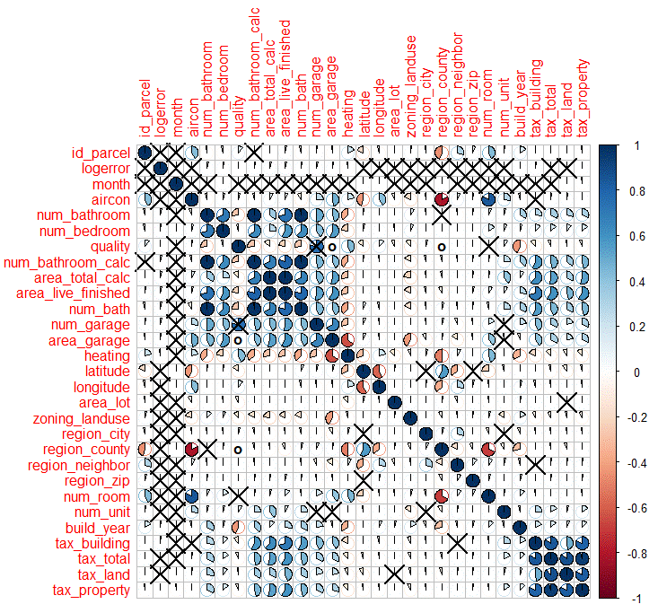
A correlation plot (corrplot) with significance is extremely useful and helps in visualizing the relationship between the numerical variables in a large dataframe as seen in the figure below. For instance, dark blue circles reveal a strong positive correlation, while dark red ones indicate a strong negative correlation between the variables. Furthermore, multi-collinear columns are highly correlated and can be easily identified from the corrplot. For instance, the tax columns (tax_building, tax_total, tax_land and tax_property), area (area_total_calc, area_live_finished) and bathroom (num_bathroom, num_bathroom_calc, num_bath) are highly correlated in this dataset. Interestingly, there is a strong negative correlation between aircon and region_county. Cells marked with ‘X’ highlight an insignificant relationship with 95 % confidence.

Figure 3: Correlation Plot with Significance

2 EDA: tableplot

The team applied another powerful visualization tool, tableplot, to explore the dataset. As shown in the figure below, different independent variables were plotted against the dependent variable logerror, with the intention of catching potential patterns between them. which could in turn give us insights on training machine learning models. Some independent variables, most notably “build_year,” showed a C shaped pattern. This indicates that the price of newer houses are more accurately estimated by Zillow than older houses, and therefore having a lower absolute logerror. Some other independent variables such as num_bathroom, area_total_calc and tax_total, showed a slightly overall increasing trend, suggesting weak positive correlations between logerror and these variables. Interestingly, these independent variables turned out to be top important variables on our models to predict logerror.

Figure 4: Tableplot of Independent Variables vs Logerror

3 Data Imputation

The original dataset has a lot of missing values. Imputation is very important during the whole process. The team used two different ways to impute the dataset.

3.1 Round 1

The first round data imputation was performed analyzing each variable individually by looking at its missingness, type and common sense. The imputation strategies are shown below:

1. Variables with missingness greater than 95% were discarded.
2. By inspecting the correlation plot, we found some variables are correlated to each other. For correlated variables, we only kept the one with the least missingness and discarded the others.
3. For variables with values either ‘True’ or NAs, we imputed ‘True’ with 1 and NAs with 0 and made it factors.
4. For some variables with more than 2 levels, we imputed randomly with the top 4 dominant levels.
5. For total tax and total area, we imputed with the mean value.
6. For other variables we had no specific imputation strategy, we imputed randomly. 

3.2 Round 2

In an attempt to improve the prediction accuracy, following strategy was employed for imputation in the second round:

1. -999 to impute the NA of numeric columns.
2. -1 to impute the NA of categoric columns.
3. Change some categorical columns to numeric columns.
4. Scale all the dataset.

4 Machine Learning Models & Results

4.1 Logic based methods

In supervised machine learning, the objective is to predict some dependent variable Y in terms of several independent variables:

Y=f(x1,x2,x3,....xn)

Specifically for the Zillow competition, the above equation can be expressed as follows:

logerror=f(month,tax,year built,...)

In order to understand the given data before running Machine Learning algorithms, Team Entropy decided to focus simply on the given values of logerror and looked at the statistics (see density plot below). In the first model analyzed, the mean value of logerror was used as the predicted values for logerror for the entire dataset. Interestingly, even such a simple model produced a Kaggle score of 0.0651279 which is significantly better than more sophisticated Machine Learning Models. In the second model, predictions for the logerror were made by randomly sampling the probability density of the unknown logerror values. Although it is reasonable to assume that the distribution of logerror in the training set would be similar to the complete dataset, random sampling resulted in a poor model and the Kaggle score was 0.1075059.

Figure 5: Distribution of Logerror and Basis for Logic Based Models

4.2 Elastic net regularization (Ridge and Lasso)

After getting a sense of the data based on Exploratory Data Analysis and predictions from logic based methods, Team Entropy decided to hierarchically include more complexity in our models. It is well known that the coefficients obtained using linear models help understand the relationship between the dependent variable and each of the independent variables. Furthermore, the mean value based prediction discussed in the previous section is a special case of linear model having only the intercept term. In order to determine the linear model, the package ‘glmnet’ was employed in R, that essentially minimized the following function:

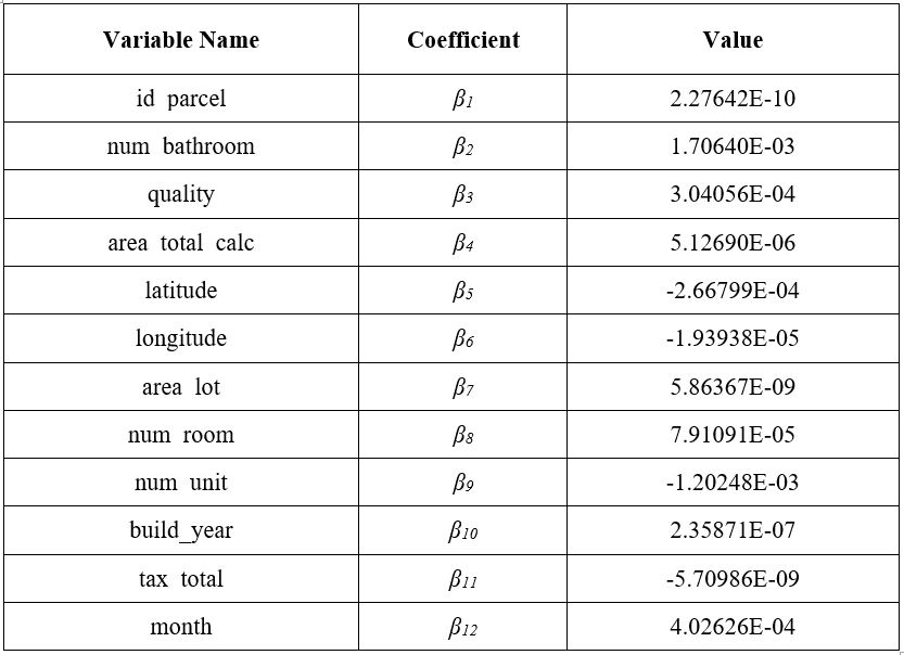
where, y_i is the element of logerror, x_i is the independent variable, and 0 represent the coefficients and the intercept of the linear model, respectively. N is the number of observations (rows in the dataframe), p is the number of independent variables (columns in the dataframe). The variables and are the hyper-parameters. Setting α=0, results in Ridge regression, while setting it as 1 corresponds to the Lasso model. Any other choice of between 0 and 1 corresponds to an  Elastic net regularization. The best choice for the hyper-parameter is determined through a grid search along with a 10-fold cross-validation (see Figures 4 and 5). The resulting relationship using a Lasso model is summarized in TABLE-1. This particular model had a Mean Absolute Error of 0.05723179 and the resulting Kaggle score was 0.0649128.

Figure 6: Effect of the Hyper-parameter  λ on the Lasso Coefficients

Figure 7: Effect of Hyper-parameter λ on the Mean Square Error

TABLE 1: Coefficients based on a Lasso Model

4.3 Random forest

Random forest is a popular machine learning algorithms extensively used in industries. It’s capable of dealing with both regression and classification problems and can be used for unsupervised machine learning as well. The training algorithm grows a number(controlled by ntree) of decision trees in which at each node only a subset of independent variables(controlled by mtry)  are considered for splitting. By randomly sampling rows(bagging) and columns (mtry), the trees generated are not correlated to each other. The result is reduced variance (nodesize and maxnodes control the variance of single tree) when the average of the trees are taken for prediction.

To train random forest model to predict logerror, a 3 fold cross validation grid search was performed on the hyperparameter mtry on training set from our 1st round imputation and cleaning. With 23 uncorrelated independent variables, the mtry that gave lowest MAE score was 4(Figure below), which agrees with the rule of thumb of choosing square root of total number of independent variables. However, when the grid search of mtry was performed on the training set from our second round imputation, the best mtry turned out to be 2. We interpret that this is due to the fact that almost all the independent variables(only dropped two columns containing large unique of character levels) were kept in the training set 2. If a larger mtry number was to be used, several important and correlated independent variables such as area and tax related variables would have a high chance to be picked up in many trees making the trees correlated to each other. This would cause the model to be easily overfitted. Therefore, a small mtry number was needed to keep the trees uncorrelated to each other.

Figure 8 : Grid Search of mtry. Left:  Grid Search of mtry of Training Set from 1st Round Imputation and Cleaning; Right: Grid Search of mtry of Training set From 2nd Round Imputation and Cleaning

A search of MAE scores with different number of trees was then performed with the best mtry found above. The result shows that the default number 500 seems to be a reasonable choice, as the gain on the decreasing of MAE diminish after 500 trees. However, in the context of Kaggle competition where the ranking are solely based on accuracy of the prediction, 800 trees were used eventually as it’s the maximum number that our computer was able to handle.

Figure 9: MAE Score with Different Number of Trees

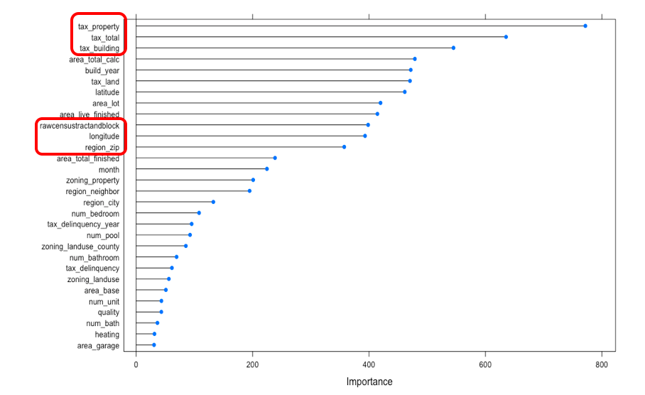
The importance of variables in the final model was visualized in an importance plot shown below. Build_year, tax related features, num_bathroom and num_bedroom were among the top of the list. These independent variables play more important role in predicting logerror, and may contain information/patterns that Zillow overlooked in its Zestimate model.

Figure 10: Importance Plot of Different Features

4.4 Gradient Boosting

Gradient boosting is a very useful machine learning technique for regression and classification problems, which produces a prediction model in the form of an ensemble of weak prediction models, typically decision trees. It builds the model in a stage-wise fashion like other boosting methods do, and it generalizes them by allowing optimization of an arbitrary differentiable loss function.

The team used gradient boosting model for the first and second imputation dataset. Here is one of the grid search result for the first imputation.This is the comparison of variable importance of two imputation dataset. So the team can find the result that second round imputation works for gbm model. A lot of variables are considered by gbm model compared with the result of the first round imputation.

Figure 11: Importance Plot of Different Features--Round 1 Imputation
Figure 12: Importance Plot of Different Features--Round 2 Imputation

The team submitted to Kaggle four times using gbm. These are the parameters for round 1 and round 2 imputations and the right plot is the Kaggle MAE for each submission. This left one is the parameter of our best score using round 1 and round 2 imputation dataset. And the right one is Kaggle MAE score of each time. 

Figure 13: Parameters & Kaggle MAE Score

4.5 XGBoost

Based on gradient boosting framework, XGBoost is an optimized gradient boosting library. It is enabled with parallel processing, which makes XGBoost at least ten times faster than any other tree based models. Regularization is provided in XGBoost to avoid overfitting. Another advantage of XGBoost is flexibility. Regression, classification, and user-defined objective functions are supported. An objective function is applied to measure the performance of the model given a certain set of parameters. User defined evaluation metrics are supported as well. Missing values are handled internally by the model so that it runs with the raw data.

In the project, the team first inputted the original dataset into XGBoost model and the importance matrix is shown below. Based on the importance matrix and the first round imputation results, the team then ran the model with the cleaned dataset of 22 variables. The importance matrix generated using cleaned dataset is consistent with the model run by original data. However, compared to RandomForest and GBM which put all tax variables at important places, XGBoost omitted the tax variables. The team then ran XGBoost on the second round cleaned data. One-hot encoding was also applied. It converts the categorical variables into numeric by creating dummy variables for each level of categorical variables. One-hot encoding aims to generate new features thus increase the accuracy of the model.

Looking at the Kaggle scores shown below, the best performance was given by the first round cleaned data. This proves the effectiveness of our first round data imputation. On the other hand, the second round data imputation and the one-hot encoding did not perform well.

Figure 14: Feature Importance of Original Data and  1^st  Round Cleaned Data

4.6 Automatic Machine Learning (h2o)

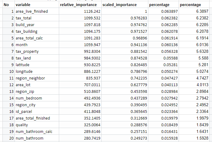
The automl package from h2o possibly presents a perspective on the future of Machine Learning. The package automates Machine Learning to the extent that there is no need to clean up the dataframe or to decide on the modeling strategy. The automl package runs a slew of Machine Learning algorithms on the entire dataframe and summarizes the top models in a leaderboard (see TABLE 2). For this specific problem, automl predicts that the Distributed Random Forest (DRF) is the best performing algorithm. The important variables for the DRF model is summarized in TABLE 3 and the corresponding Kaggle score was 0.0649128.

TABLE 2: Leaderboard in the Automl Package

TABLE 3: Variable Importance in the DRF Mode

5 Conclusions

In the course of this project, Team Entropy implemented a variety of Machine Learning algorithms for predicting the logerror. In Figure-15, we compare the performance of various models for the months October to December. It can be seen predictions from XGB and Lasso are pretty much flat highlighting that the monthly change in the logerror values are not captured in these models. The Random Forest as well as the GBM models are able to capture some trend in logerror as a function of months. Hence, it is not surprising that GBM was our best performing model on Kaggle followed by Random Forest, although all models predict significantly lower values for logerror for these three months.

Figure 15: Model Comparison

The team members collaborated equally throughout the entire project. EDA was performed to examine the structure and degree of missingness of the raw data. Imputations were being made while the models were running. First round imputation was done by studying each variable individually by looking at the type, missingness percentage, and common sense. In the second round imputation, a different strategy was employed; numerical NAs were imputed with -999 and the categorical NAs were imputed with -1. Five models were trained, which include Lasso, Random Forest, Gradient Boosting Machine, XGBoost and H2O. The best results of each model are shown below:

TABLE 3: Best Scores of Each Model

The best performance was given by GBM with the second round imputed data. The Kaggle ranking at the time of submission was 725^th. The second-best result was given be Random Forest with the ranking of 753^rd at the time of submission.

6 Future Work

The following ideas can be explored in the future to improve the prediction accuracy and thereby the Kaggle rank:

• Improve the current model by fine tuning the hyperparameters
• Generate appropriate features using feature engineering
• Use of stacking to combine models for improved prediction accuracy

References

[1] Samuel, A. (1959). Some studies in machine learning using the game of Checkers. IBM Journal of Research and Development, 3 (3), 211–229